OPEN JOURNAL OF ATMOSPHERIC AND CLIMATE CHANGE
ISSN(Print): 2374-3794 ISSN(Online): 2374-3808
In Press
OPEN JOURNAL OF ATMOSPHERIC AND CLIMATE CHANGE
Advanced Two-Layer Climate Model for the
Assessment of Global Warming by CO2
Hermann Harde*
Experimental Physics and Materials Science, Helmut-Schmidt-University, Hamburg, Germany.
*Corresponding author: harde@hsu-hh.de
Abstract:
We present an advanced two-layer climate model, especially appropriate to calculate the
influence of an increasing CO2-concentration and a varying solar activity on global warming.
The model describes the atmosphere and the ground as two layers acting simultaneously as
absorbers and Planck radiators, and it includes additional heat transfer between these layers due
to convection and evaporation. The model considers all relevant feedback processes caused by
changes of water vapour, lapse-rate, surface albedo or convection and evaporation. In particular,
the influence of clouds with a thermally or solar induced feedback is investigated in some detail.
The short- and long-wave absorptivities of the most important greenhouse gases water vapour,
carbon dioxide, methane and ozone are derived from line-by-line calculations based on the
HITRAN08-databasis and are integrated in the model. Simulations including an increased solar
activity over the last century give a CO2 initiated warming of 0.2 ° C and a solar influence of
0.54 ° C over this period, corresponding to a CO2 climate sensitivity of 0.6 ° C (doubling of CO2)
and a solar sensitivity of 0.5 ° C (0.1 % increase of the solar constant).
Keywords:
Carbon Dioxide; Climate Model; Climate Sensitivity; Cloud Cover; Global Warming; Solar Activity
1. INTRODUCTION
Understanding of recent changes in the climate system results from combining observations, studies of
feedback processes, and model simulations [1]. Although the substantiated state of knowledge about the
Earth-atmosphere system (EASy) could significantly be improved over the last decade, explanations of the
observed global warming over the last century are quite manifold and contradictory. One reason might be
that quite different and even counteracting processes control our climate, and it is not always clear what
individual contribution they have. The weighting of these processes in model simulations have significant
consequences on the implications what really determines our future climate.
Many climate models, particularly the Atmosphere-Ocean General Circulation Models (AOGCMs) [2]
were developed not only to simulate the global scenario, but also to predict local climate variations and this
as a function of time. Therefore, they have to solve a dense grid of coupled nonlinear differential equations
depending on endless additional parameters, which make these calculations extremely time consuming
and even instable. So, smallest variations in the initial constraints or corrections on a multidimensional
1

OPEN JOURNAL OF ATMOSPHERIC AND CLIMATE CHANGE
parameter platform already cause large deviations in the final result and can dissemble good agreement
with some observations but with completely wrong conclusions.
For the actual assessment of one of the most fundamental quantities in climate sciences, the equilibrium
climate sensitivity, representing the temperature increase at doubled CO2 concentration [2], p.629, the
Intergovernmental Panel on Climate Change (IPCC) favours the concept of radiative forcing (RF), which
is supposed to be appropriate to describe the transition of the surface-troposphere system from one
equilibrium state to another in response to an externally imposed perturbation. However, generally this
concept only describes a 1st order approximation on such external perturbation [3], p.354. So, it is
assumed that with increasing greenhouse (GH) gas concentration additionally absorbed radiation in a first
step only causes a temperature increase of the atmosphere up to a level, at which the atmosphere just can
release the additional absorption as increased radiation energy to space. A feedback to the Earth's surface
is then supposed as linear response to the perturbation, where the increased atmospheric temperature
is simply transposed one to one to the surface without considering significant interrelations between
both layers, generally causing a completely new radiation and energy balance after the perturbation. So,
convection and evaporation processes are directly temperature dependent, and any radiation flux varies
strongly nonlinear with the 4th power to the temperature. All this modifies the amount of re-absorbed
radiation in the atmosphere and the direct radiation losses to space. Thus, the response of EASy on any
perturbation cannot be deduced from the temperature response of the atmosphere alone, but has to satisfy
the energy balance at the surface as well as at the top of the atmosphere (TOA), which results in a new
thermal equilibrium of EASy.
In contrast to the RF-concept and the extremely complex AOGCMs here we present an advanced two-
layer climate model, especially appropriate to calculate the influence of increasing CO2 concentrations
on global warming as well as the impact of solar variations on the climate. The model describes the
atmosphere and the ground as two layers acting simultaneously as absorbers and Planck radiators, and it
includes additional heat transfer between these layers due to convection and evaporation. At equilibrium
both, the atmosphere as well as the ground, release as much power as they suck up from the sun and
the neighbouring layer. An external perturbation, e.g., caused by variations of the solar activity or the
GH-gases then forces the system to come to a new equilibrium with new temperature distributions for the
Earth and the atmosphere.
The model includes short- (sw) and long-wave (lw) scattering processes at the atmosphere and at clouds,
in particular it considers multiple scattering and reflection between the surface and clouds. It also includes
the common feedback processes like water vapour, lapse rate and albedo feedback, but additionally takes
into account temperature dependent sensible and latent heat fluxes as well as a temperature induced and
solar induced cloud cover feedback.
While propagation losses of radiation in the atmosphere are generally expressed by a radiative forcing
term, we trace any changes of GH-gas concentrations back to the sw and lw absorptivities of these gases,
which therefore, represent the key parameters in our climate model. These absorptivities are calculated
for the most important GH-gases water vapor, carbon dioxide, methane and ozone and are derived from
line-by-line calculations based on the HITRAN08-database [4]. Since the concentration of the GH-gases
and the atmospheric pressure are changing with temperature and altitude, these calculations are performed
for up to 228 sub-layers from ground to 86 km height and additionally for three climate zones, the tropics,
mid-latitudes and high-latitudes. Finally, to determine, how these absorptivities change with the CO2
concentration, all these calculations, for the sub-layers and climate zones, are repeated for 14 different
concentrations from 0-770 ppm at otherwise same conditions.
2

Advanced Two-Layer Climate Model for the Assessment of Global Warming by CO2
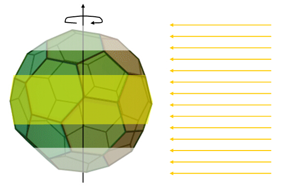
The changing path length of sun light in the sub-layers, which depends on the angle of incidence to the
atmosphere and, therefore, on the geographic latitude and longitude, is included by considering the Earth
as a truncated icosahedron (Bucky ball) consisting of 32 surface elements with well defined angles to the
incident radiation, and then assigning each of these areas to one of the three climate zones.
The propagation of the long-wave radiation, in particular the up- and down-welling radiation emitted
by the atmosphere itself, as well as changes of this radiation with temperature are derived from radiation
transfer calculations [57] for each zone.
The sw spectral absorptivity, reflecting the solar absorption, is calculated over a spectral range from
0.18 ľm, and the lw spectral absorptivity, characterizing the absorption of the terrestrial and atmospheric
radiation, is computed from 3100 ľm. Both these spectra show significant saturation with increasing
concentration of water vapour and CO2 as well as strong mutual interference of these spectra. We
explicate, how both effects essentially attenuate the response of the climate system on a changing CO2
concentration.
The sw and lw absorptivities are integrated in our climate model to simulate the Earth's surface temper-
ature and the lower tropospheric temperature as a function of the CO2 concentration. The temperature
increase at doubled CO2 concentration then directly gives the CO2 climate sensitivity and the respective
air sensitivity.
Different scenarios, under clear sky conditions and regular cloud cover, are extensively investigated,
including all relevant feedback processes and also the influence of a changing solar activity. These
investigations show the dominant impact of a varying cloud cover on global warming, caused by a
thermally induced and/or solar induced cloud feedback. In particular, they indicate, that due to this strong
cloud feedback the observed warming over the last century can only satisfactorily be explained, attributing
a significant fraction to the increased solar activity over this period.
Our simulations predict a climate sensitivity CS = 0.6 ° C and a solar sensitivity SS = 0.5 ° C (0.1 %
change of the solar constant), whereas the IPCC specifies in its actual assessment report [1] the equilibrium
climate sensitivity to be likely in the range 1.5 ° C to 4.5 ° C (66-100 % probability with high confidence)
and extremely unlikely less than 1 ° C (0-5 % with high confidence).
2. SPECTROSCOPIC CALCULATIONS
The influence of GH-gases on EASy is almost exclusively determined by the absorption and emission
of these gases in the atmosphere. Therefore, the respective absorption and emission spectra represent
the key parameters in any climate model. For the most important GH-gases water vapour, carbon
dioxide, methane and ozone the sw and lw absorption is derived from line-by-line calculations based on
the HITRAN08-database [4]. Other infrared active gases like N2O, SF6 or the halogen-hydrocarbons
(halocarbons) with significantly lower concentrations in the atmosphere have no noticeable influence on
the further investigations.
Because of the different temperatures and the water content in the atmosphere three climate zones
are distinguished: the tropics with an average temperature of 26 ° C, the mid-latitudes with 8 ° C and the
high-latitudes with -7 ° C.
In this section we briefly explain the underlying principles of our spectral calculations and present the
results for the sw and lw absorptivities, in particular the mutual interference of water vapour and carbon
3

OPEN JOURNAL OF ATMOSPHERIC AND CLIMATE CHANGE
dioxide with their respective influence on the total absorption.
2.1 Fundamentals
2.1.1 Integral Absorptivity
The spectral intensity of well collimated radiation, transmitting a gas sample, is given by Lambert-Beer's
law [5, 6]:
I (r) = I (0) ˇ e-( ,r)
(1)

where I (0) is the initial spectral intensity on the wavelength

and ( ,r) the optical depth. In the
simplest case ( ,r) is just the product of the absorption coefficient ( ) of the gas and the path length
r. Under atmospheric conditions, however, ( ) is varying over the propagation length due to pressure
and temperature changes with altitude (z-direction, perpendicular to the surface). Then ( ,r) has to
be expressed as an integral of ( ,r) over the path length L. In addition, ( ,r) generally reflects the
absorption at , caused by different molecular transitions and different gases in the atmosphere. Therefore,
( ,r) assumes the more general form:
L
L
i
( , L) =
( , z(r))dr =
Ż (
(
nm , pip z(r)), pt (z(r)), T (z(r)))dr
(2)
k
0
0
where Ż i
nmrepresents the effective absorption coefficient, expressing the difference between induced
absorption and induced emission processes on an optical or infrared transition between a lower molecular
state n and an upper state m [7, 8]. The superscript i distinguishes between the different gas components
in the atmosphere. pi (
p z(r)) is the partial pressure of the i-th gas, pt (z(r)) the total pressure, T (z(r)) the
temperature at altitude z and L the path length in the atmosphere. Summation over k expresses the sum
over the different transitions and gases.
The integral in (2) is solved numerically by segmenting the atmosphere into up to 228 layers, then
calculating the optical depth of each individual layer under the actual conditions at that altitude, and
finally summing up over all layers.
The spectral absorptivity also follows from Lambert-Beer's law as:
I (L)
a (L) = 1 - t (L) = 1 -
= 1 - e-( ,L)
(3)

I (0)

which describes the relative absorption on the wavelength or frequency = c/ . t is the respective

spectral transmissivity and c the speed of light. Then, with (3) the total or integral absorptivity can be
defined as:
I (0) ˇ a (L) d
a(L) = 0

× 100 [%]
(4)
I (0) d
0

This quantity is quite appropriate to express any radiation losses and by this the absorbed power in the
atmosphere over the path length L. Once, calculated for a gas mixture and the respective sw or lw spectral
4

Advanced Two-Layer Climate Model for the Assessment of Global Warming by CO2
distribution I , the absorptivity can quite universally be used to simulate the influence of the gas mixture

on the radiation and energy balance of EASy. Therefore, the absortivities aSW for the sw solar radiation
and aLW for the lw terrestrial radiation are the key parameters to determine the influence of an increasing
CO2 concentration on global warming.
2.1.2 Atmospheric Pressure and Temperature Changes
The interaction of radiation with gases is considered up to an altitude of 86 km. For the pressure and
temperature variations over this altitude we orientate at the US Standard Atmosphere model [9], but
introduce some smaller modifications for the individual climate zones Z. The standard model uses a
global mean ground temperature of 15 ° C, and a lapse rate of 6.5 ° C/km over the troposphere up to the
tropopause, yielding a temperature of 216.65 K in 11 km altitude. However, the ground temperatures
T Zone(0) of the three zones approximately change over 33 ° C (tropics: 26 ° C = 299.15 K; mid-latitudes:
8 ° C = 281.15 K; high-latitudes: -7 ° C = 266.15 K), whereas at the tropopause the temperatures almost
have assimilated to each other (see also subsection 5.4). Therefore, we use a slightly different temperature
variation over the troposphere for each of the three climate zones:
T Zone(0) - 216.65 K
T Zone(z) = T Zone(0) -
z
(5)
11, 000 m
with the respective lapse rates:
T
T Zone(0) - 216.65 K
lZone = -
=
r
(6)
z
11, 000 m
Due to the different temperature variations and lapse rates also different pressure variations over the
troposphere have to be distinguished for the three zones:
Mˇg
lZone(z - z0) RˇlZone
r
pZone(z) = p(z
r
0)
1 -
(7)
T (z0)
with M = 0.02896 kg/mol as the molar mass of the atmosphere, g = 9.81 m/s2 as gravitational acceleration,
R = 8.314 J/K/mol as universal gas constant and z0 as reference altitude.
Over the tropopause, the stratosphere and mesosphere again the standard atmosphere model is applied.
2.1.3 Concentration of Greenhouse Gases
Carbon dioxide and methane are well mixed gases in the atmosphere, which are found in almost
constant concentrations over the surface and the altitude. Therefore, their number densities, which are
important for the absorption strength on a molecular transition, vary proportional with pressure and
reciprocal with temperature. Within this paper we use a reference concentration for CO2 of 380 ppm and
for CH4 of 1.8 ppm.
Ozone is distributed over the whole stratosphere and tropopause with a maximum concentration of 7
ppm around an altitude of 38 km and extending in downward direction almost down to the troposphere, in
upward direction up to the mesosphere.
5

OPEN JOURNAL OF ATMOSPHERIC AND CLIMATE CHANGE
More complicated but also much more important for the energy and radiation budget in the atmosphere
is the water vapour content. It is almost exclusively found in the troposphere up to an altitude of 11 km,
and due to the Clausius-Clapeyron-equation its concentration strongly depends on the temperature, which
on the one hand side changes with altitude above ground and on the other hand significantly varies with
latitude.
From GPS-measurements [10], by which the integral water content in the three climate zones can be
determined, together with the temperature and pressure dependence we can calculate the water vapour
concentration as a function of altitude (for details see [11]). The mean concentration is in good agreement
with the Average Global Atmosphere, but almost 2x larger than the data derived from the US Standard
Atmosphere [9], which is only valid for mid-latitudes. The respective graphs for the saturated and
unsaturated partial pressures are shown in Figure 1. These vapour variations as a function of altitude
form the basis for the further spectroscopic calculations.
Figure 1. a) Water vapour concentration in the tropics at 26 oC, b) mid-latitudes at 8 oC and c) high-latitudes at -7
oC as a function of altitude.
6

Advanced Two-Layer Climate Model for the Assessment of Global Warming by CO2
2.2 Short-Wave Absorption in the Atmosphere
2.2.1 Path Length in the Atmosphere
Sun light entering the Earth's atmosphere can be considered as a well collimated beam, but due to the
spherical shape of the Earth the angle of incidence on an individual gas layer varies with latitude and
longitude over 90 ° and by this also the path length, over which absorption within the layer takes place.
In order to restrict the calculations to a finite number of angles and propagation lengths, the earth is
considered as a truncated icosahedron (also known as Bucky ball) consisting of 12 pentagonal and 20
hexagonal surface elements (see Figure 2).
Figure 2. The globe as Bucky ball.
When turning the Bucky ball to a position that a pentagonal area is oriented perpendicular to the
incident sun light, further pentagonal and hexagonal areas with specific orientation angles to the sun can
be distinguished and respective fractions of them assigned to the three climate zones.
So, as listed in Table 1, four different areas contribute to the tropics, three to the mid-latitudes and two
to the high-latitudes. Therefore, altogether nine separate calculations, differing in their path lengths and
their conditions in the three climate zones, are necessary to determine the sw absorptivities.
While the last column in Table 1 represents the sum of the individual areas for one zone (the total sum
gives half the globe surface), for the power irradiating one specific climate zone, the respective projection
areas perpendicular to the incident radiation have to be considered.
Table 1. Assigned icosahedron surfaces to the climate zones.
angle of incidence
90 ° - P
52.9 ° - H
25.5 ° - P
11.6 ° - H
area (1012 m2)
tropics
1.0
3.5
2.0
1.5
127.8
mid-latitudes

1.5
2.5
2.5
103.5
high-latitudes

0.5
1
24.4
path in atmosphere (km)
86
108.2
206
535.1
255.8
7

OPEN JOURNAL OF ATMOSPHERIC AND CLIMATE CHANGE
2.2.2 Absorption Spectrum
Our calculations of the solar absorption in the atmosphere cover a spectral range of 0.18 ľm and
are based on the HITRAN08-database [4]. Within this spectral interval 60, 994 water lines, 262, 104
methane lines, and 234, 210 carbon dioxide lines are found. Exact calculations with these more than
500, 000 lines only contribute to an increased absorption of 0.2% compared to computations with only the
main isotopologues and with spectral line intensities larger than 10-24 cm-1/(moleculesˇcm-2). Since
this small "offset" is of no concern for further investigations of the CO2 climate sensitivity, most of the
calculations were performed with the reduced number of lines. Within the specified spectral interval this
gives for CO2
4, 421 lines, for CH4
46, 208 lines, and for H2O
9, 565 lines.
Since the HITRAN08-database does not include ultraviolet transitions of ozone, we suppose for this
gas a continuous absorption between 0.1 and 0.35 ľm with 8 %. This absorption does not interfere with
other contributions of water vapour, CO2 or CH4 and is considered separately in the climate model.
The actual spectral calculations, retrieving all the necessary parameters of a molecular transition from
the HITRAN08-database and further computing the absorption strength as well as the lineshape for
each spectral line as a function of the partial pressures, the total pressure and the temperature over the
propagation length, is done by the program platform MolExplorer [12].
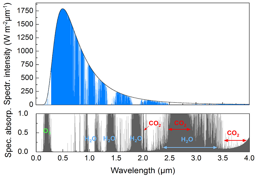
Figure 3 gives an overview over the transmission and absorption spectrum from 0 - 4 ľm, in this case
for the tropics and for perpendicular incidence of the radiation. The spectral solar intensity I can well be

approximated by a Planckian blackbody radiator of 5778K in good agreement with the observed solar
spectrum. It is represented as dotted line in the upper plot and forms the envelope of the transmitted
spectrum. The sharp dips and broader white regions indicate the strong absorption at these wavelengths,
whereas the lower plot directly represents the respective spectral absorptivity.
Figure 3. Absorption of sun light in the tropics by H2O, CO2, O3 and CH4. Above: transmission-, below:
absorption-spectrum.
This figure already shows the dominant influence of water vapour over wider spectral regions which
alone already contributes to an integral absorptivity of 13.1 %, while CO2 only causes 2.24 % and CH4
8

Advanced Two-Layer Climate Model for the Assessment of Global Warming by CO2
0.22 %. However, with water vapour, that portion which can be attributed to CO2 and CH4 (together
2.45% at standard conditions) reduces to about one quarter of the previous values. The reason is that their
absorption bands are strongly overlapping with those of water vapour, so that only 0.52 %, i.e. less than 4
% of the total absorption, can be allocated to carbon dioxide.
We have calculated the sw absorptivities for the three climate zones and also for different CO2
concentrations from 0-770 ppm, as listed in Table 2. The data of each climate zone and each concentration
already represent a weighted average over the projection areas, which contribute to a zone (see Table 1).
All spectra and by this the respective absorptivities were calculated with a spectral resolution of 1 GHz or
even better.
Table 2. sw absorptivities as a function of the CO2 concentration.
sw absorptivities asw(%)
CO2 (ppm)
tropics
mid-latitudes
high- latitudes
global
0
14.628
12.674
12.267
13.613
35
14.842
12.949
12.658
13.868
70
14.912
13.045
12.800
13.956
140
15.012
13.175
12.974
14.075
210
15.086
13.266
13.092
14.160
280
15.146
13.340
13.182
14.228
350
15.196
13.400
13.255
14.285
380
15.217
13.425
13.284
14.308
420
15.242
13.455
13.319
14.336
490
15.281
13.501
13.373
14.379
560
15.317
13.542
13.420
14.418
630
15.349
13.580
13.461
14.454
700
15.378
13.614
13.498
14.485
770
15.406
13.645
13.533
14.515
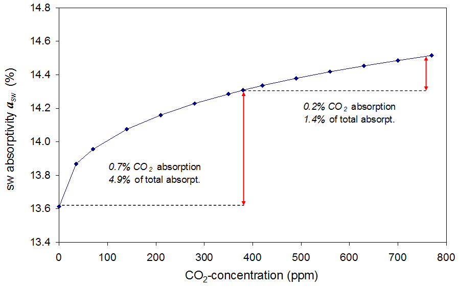
Figure 4. Global sw absorptivity as a function of the CO2 concentration caused by water vapour, CO2and CH4.
The last column in Table 2 shows the global mean values as the weighted average over the three climate
zones. This global sw absorptivity is plotted in Figure 4 as a function of the CO2 concentration and is
used in this form for the further climate simulations. It is obvious, that with increasing concentration
the absorption already shows stronger saturation, which in this case means, that within some spectral
9

OPEN JOURNAL OF ATMOSPHERIC AND CLIMATE CHANGE
regions the atmosphere already becomes completely opaque and only weaker absorption bands or lines
can further contribute to an attenuation. So, from zero to 380 ppm CO2 the absorption increases by 0.7 %,
whereas a further doubling of CO2 only contributes to less than 0.2 %.
2.3 Long-Wave Absorption in the Atmosphere
2.3.1 Spectral Range and Number of Lines
The Earth's surface and the atmosphere, both with temperatures roughly between -20 and 30 ° C,
represent Planckian radiators, which release part of their collected energy in form of lw radiation, but also
strongly absorb radiation over the infrared wavelength range. In this subsection we focus on the question,
how much of the emitted terrestrial radiation can be absorbed by the atmosphere.
For our spectral calculations we consider a range from 3-100 ľm, in which the HITRAN08-database
has stored 18, 539 water vapour lines, 178, 206 methane lines, 167, 755 carbon dioxide lines, and 284, 647
ozone lines. Again restricting the calculations on the main isotopologues and transitions with spectral
intensities larger than 10-24 cm-1/(moleculesˇcm-2), for water vapour 2, 962 lines, for CH4 17, 776 lines,
for CO2 4, 454 lines, and for O3 75, 382 lines are left. So, altogether almost 96, 000 lines are included in
the further investigations. The spectral resolution is again better than 1 GHz, and the vertical resolution
over the atmosphere with up to 228 sub-layers varies from 100 m over the troposphere up to 1.6 km in the
upper mesosphere.
2.3.2 Propagation of Terrestrial Radiation
Different to the well collimated solar radiation transmitting the atmosphere, terrestrial radiation is
emitted by each surface element of the Earth into a solid angle of 2 and is spreading out over the whole
hemisphere. In order to determine the absorption of radiation, which is propagating under different
directions and covering different distances before exiting an atmospheric layer of thickness dz, it is
necessary first to consider the interaction of an individual ray with the gas before integrating over all
directions.
Supposing the Earth's surface as a Planckian radiator with Lambertian emission, then such an individual
beam may be characterized by the spectral radiance I
ˇcos
,
ˇ d emitted under an angle to the
surface normal and into the solid angle interval d with [6, 7]
2 h c2n3
1
I
cos d =
cos d
(8)
,
h c
5
e kTE - 1
where h is Planck's constant, c the vacuum speed of light, n the refractive index, k the Boltzmann constant
and TE the Earth's surface temperature. This ray covers a distance dz / cos before leaving the layer and,
therefore, suffers from absorption losses ( ) I
ˇcos
,
/ cos ˇ d ˇdz. Then, integration over gives
(see also Ref.[7], (54)):
2
dI
cos

d
cos
,

= -
i
Ż ( , z)
I
d = -2( , z) ˇ ˇ I
(9)
dz
nm
, cos
,
k

0
10

Advanced Two-Layer Climate Model for the Assessment of Global Warming by CO2
where ( ,z) may represent the sum over the effective absorption coefficients of the involved transitions
and gases at wavelength (see (2)). Since the integral I
ˇcos
in (9) just defines the
,
d = ˇI ,
spectral intensity I (or spectral flux density) representing the mean expansion of the emitted radiation

perpendicular to the surface in z-direction, (9) can be written as
dI (z)

= -2( , z) ˇ I (z)
(10)
dz

This differential equation for the spectral intensity shows that the effective absorption coefficient is
twice that of the spectral radiance, or in other words the average propagation length of the radiation to
pass the layer, is twice the layer thickness. This means, we also can assume radiation, which is absorbed
at the regular absorption coefficient ( ,z), but in average is propagating under an angle of 60 ° to the
surface normal (1/cos 60 ° = 2).
In reality, the Earth will deviate from a Lambertian radiator and due to Mie scattering or inhomogeneities
in the atmosphere the individual rays do not obey geometric optics. Therefore, altogether it seems
reasonable to apply a slightly smaller effective absorption coefficient of (1/cos )ˇ ( ,z) in (10) with
an average propagation angle of = 52 ° . This description is in close agreement with the two-stream
approximation (see Ref. 6, p.232) and corresponds to a diffusivity factor of 1/cos . Integration of (10)
over z and applying (4) then gives the lw absorptivity aLW .
2.3.3 Absorption Spectrum
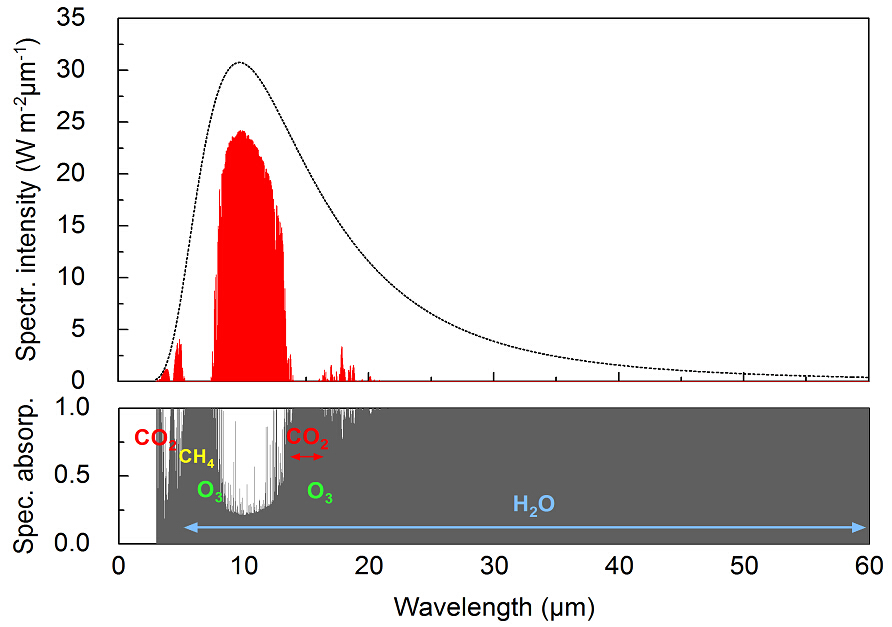
Figure 5. Transmission and absorption spectrum of the terrestrial radiation in the atmosphere.
Figure 5 shows the transmission and absorption spectrum of the terrestrial radiation from 3-60 ľm for
the tropics with a ground temperature of 26 ° C and a water vapour concentration of 2.29 %. The spectral
intensity I for a Planckian blackbody radiator of 26 ° C is plotted as dotted line. The total flux as the

integral over the spectral intensity in this case is IE = 454W /m2, from which 85.7 % are absorbed by the
11

OPEN JOURNAL OF ATMOSPHERIC AND CLIMATE CHANGE
GH-gases. Over wider spectral regions the atmosphere is almost completely opaque, only around 10 ľm
less than 15 % of the terrestrial radiation can directly be released to space. Again by far the largest amount
of the absorption results from water vapour, which already contributes to 80.1 %, whereas CO2 alone
delivers 22.9 %, CH4 2.0 % and O3 3.3 %. However, due to the overlap with the water vapour spectrum
in the presence of the other gases CO2 only causes an additional increase of the lw absorptivity of 3.5 %.
The calculated lw absorptivities for the three climate zones as a function of the CO2 concentration are
listed in Table 3. The values in the second last column again represent the weighted averages over the
three climate zones. These averages, however, slightly deviate by about 1% from calculations performed
under conditions with a unique temperature of 15.5 ° C and a unique water vapour concentration of 14,615
ppm. These values for the temperature and vapour concentration were also determined as weighted
averages over the climate zones. The absorptivities calculated with these global mean parameters are
listed in the last column of Table 3 and are plotted as a function of the CO2 concentration in Figure 6.
Table 3. lw absorptivities as a function of the CO2 concentration.
lw absorptivities aLW (%)
CO2 (ppm)
tropics
mid-latitudes
high- latitudes average 3 zones
global mean
0
81.90
69.44
58.98
74.68
77.02
35
83.80
74.48
67.04
78.43
80.08
70
84.18
75.35
68.32
79.10
80.62
140
84.65
76.31
69.80
79.86
81.29
210
84.99
77.00
70.77
80.40
81.76
280
85.28
77.51
71.52
80.83
82.14
350
85.53
77.95
72.14
81.19
82.45
380
85.65
78.12
72.38
81.34
82.58
420
85.76
78.33
72.68
81.51
82.74
490
85.97
78.67
73.16
81.80
83.00
560
86.16
78.98
73.61
82.06
83.24
630
86.35
79.29
74.02
82.32
83.46
700
86.52
79.58
74.41
82.56
83.68
770
86.69
79.85
74.78
82.79
83.88
Figure 6. Global lw absorptivity as a function of the CO2 concentration caused by water vapour, CO2, CH4 and O3.
Since in this paper we particularly focus on the global influence of CO2, characterized by the global
12

Advanced Two-Layer Climate Model for the Assessment of Global Warming by CO2
climate sensitivity, it seems appropriate to use these data for our further simulations. In any way, it is
found that for the climate sensitivity it makes no bigger difference, which data set is used.
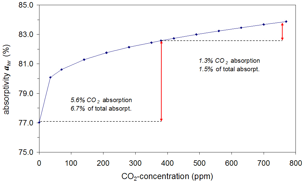
Similar to the sw absorptivities also the lw radiation suffers from stronger saturation effects with
increasing concentration. So, from zero to 380 ppm the absorption increases by 5.6% whereas a further
doubling of the CO2 concentration only contributes to about 1.3 %.
3. RADIATION TRANSFER IN THE ATMOSPHERE
In the previous section we were focusing on the absorption of solar and terrestrial radiation in the
atmosphere, both increasing the mechanical, kinetic and inner energy of the gaseous cover. But in thermal
equilibrium the atmosphere has to release the same amount of energy to space - and also some fraction
back to the surface - as it accepts by absorbed radiation and heat transfer. This mostly appears via radiation
processes in upward and downward direction, since in the same way, as GH gases are strong absorbers,
they are also strong emitters of infrared radiation.
Therefore, a more extensive analysis of the energy and radiation balance of the atmosphere not only
accounts for the net absorbed power from the incident radiation, as considered in (1)-(4) and (10), but it
also includes any radiation originating from the atmosphere itself as well as any re-radiation due to an
external excitation. This is the subject of this section.
3.1 Radiation Transfer Equation for the Spectral Radiance
When considering radiation, which transmits the atmosphere and on its way suffers from absorption
losses, this radiation simultaneously is superimposed by thermal radiation originating from spontaneous
emission of infrared active molecules in the atmosphere. Since this emission almost covers the same
wavelength range as the terrestrial radiation, it can significantly reduce the effective absorption losses of a
beam, it can modify the spectral distribution or can be the origin of new up- and down-welling radiation
in the atmosphere.
The spectral power density on the wavelength due to spontaneous emission of the different gases i on
the transitions m n into the full solid angle of 4 is:
du
hc
= hmn Ai
Ai
dt
mn Nim gi(v, mn) =
mn Nim gi( , mn)
(11)
k
k
mn
and represents a spectral generation rate of photons of energy hmn per volume. u is the spectral

energy density, mn the resonance transition frequency, mn the respective resonance wavelength, Amn the
Einstein coefficient for spontaneous emission, Nm the number density of an excited molecular state m and
g( , mn) the lineshape function of a molecular transition [7].
Therefore, over small propagation distances dr in the atmosphere both contributions, the radiation
losses and the thermal emission, can be summed up, and for the spectral radiance I
we can write:
,
dI
(r)
1
hc
,
= -
i
Ż ( ) ˇ I
(r) +

Ai
(r) gi( , mn)
(12)
dr
nm
,
4
mn Nim
k
k mn
13

OPEN JOURNAL OF ATMOSPHERIC AND CLIMATE CHANGE
While the first term is known from Lambert-Beer's law, representing the absorption and emission
processes induced by the incident radiation, the second term describes the spontaneous emission on the
different molecular transitions contributing to the spectral radiance at wavelength . Summation over k
again means the sum over individual transitions within one molecule and over the different gases indicated
by the superscript i.
Photons emerging from a volume element spread out into the neighbouring areas, but also arrive from
the neighbourhood. In a homogeneous medium both fluxes just compensate each other. Nevertheless,
in a dense atmosphere as found within the troposphere, photons have an average lifetime, before they
are annihilated due to an absorption in the gas. Of course, this is the case for the incident radiation, as
represented by the first term in (12), but in the same way this happens to the thermal background radiation.
With an average photon lifetime
n
n
1

(
(
=
ph ) = lph )
(13)
c
c Ż
i (
nm )
where l
i
ph = 1/ Ż
nm is the mean free path of a photon in the gas, before it is absorbed on the wavelength
, at thermal equilibrium we can write for the spectral energy density:
h ˇ n
Ai
u =
ˇ
mn Ni

m gi( , mn)
(14)
Ż
i (
nm )
k
mn
k
As already outlined previously ([7], subsection 2.5), u just represents the spectral energy density of a

Planckian radiator at and is given by
8 n4 hc
1
4 n
u =
=
B
(T

hc
,
A)
(15)
5
c
e kTA - 1
with B
(T
,
A) as the Kirchhoff-Planck function, which is identical with (8) but now describes the spectral
radiance of the atmosphere at temperature TA.
With (14) and (15) then the second term in (12) can be expressed by the respective absorption coeffi-
cients on a transition, times the Kirchhoff-Planck function:
dI
(r)
,
= -
i
i
Ż ( , r) ˇ I
(r) + Ż (,r) ˇ B
(TA(r))
(16)
dr
nm
,
nm
,
k
k
This equation is known as the Schwarzschild equation [57, 13], which describes the propagation of
radiation in an absorbing gas and in the presence of thermal background radiation of this gas. Generally
this equation is derived from pure thermodynamic considerations and is valid under conditions, when
the collision rate Cmn of superelastic collisions (transitions from mn due to de-exciting, non-radiating
collisions) is much larger than the spontaneous emission rate Amn. Typically this is the case within the
whole troposphere up to the stratosphere.
For our calculations from the surface up to the mesopause and vice versa we use a generalized form of
the radiation transfer equation (see Ref. 7):
dI
(r)
,
=
i
Ż ( , r) -(r) ˇ I
(r) + B
(TA(r))
(17)
dr
nm
,
,
k
14

Advanced Two-Layer Climate Model for the Assessment of Global Warming by CO2
which can also be derived from (12) and covers both limiting cases of thin and dense atmospheres. In
particular, it allows a continuous transition from low to high densities, controlled by a collision dependent
parameter (r) [7]:
1/4
(r) = 1 -
(18)
1 +Cmn(r)/Amn
which can adopt values from 3/4 1 for 0 Cmn/Amn .
3.2 Radiation Transfer Equation for the Spectral Intensity
Since for the further considerations the radiation emitted into the full hemisphere is of interest, (17) has
to be integrated over the solid angle = 2. As already discussed in subsection 2.3, a beam, propagating
under an angle to the layer normal (z-direction), only contributes an amount I
cos
,
ˇ d to the
spectral intensity due to Lambert's law. The same is assumed to be true for the thermal radiation emitted
by a gas layer under this angle.
On the other hand the path length through a layer of depth dz is increasing with dr = dz/cos , so that
the -dependence for both terms I
and B
disappears.
,
,
Therefore, analogous to (9) integration of (17) over and using the identities I =
as well as

ˇI ,
B =
, gives for the spectral intensity in z-direction:

ˇB ,
dI (z)

= 2
i
Ż ( , z) -(z)I (z) + B (TA(z))
(19)
dz
nm

k
Since the density of the gases, the total pressure and the temperature are changing with altitude, (19)
has to be solved stepwise for thin layers of thickness
i
z, over which the absorption coefficients Ż
nm ,
and the spectral intensities I
and B can be assumed to be constant. With the running index j for

different layers then (19) can be calculated stepwise by (see Ref. 7, subsection 4.5):
j
j-1
j
i, j
1
j
j
j
i, j
I ( z) = I
e-2 Żnm( )z +
B (T ) ˇ (1 - e-2 Żnm( )z)
(20)

A
j

The intensity in the
j-1
j-th layer is computed from the previous intensity I
of the (j-1)-th layer with

the values Ż i, j
j
j
nm( )and B (T ) of the j-th layer. In this way the propagation over the full atmosphere is

A
calculated stepwise.
The first term in (20) describes the transmission of the incident spectral intensity in a lossy medium
over the layer thickness, whereas the second term represents the self-absorption of the thermal background
radiation in forward direction and is identical with the spontaneous emission of the layer into one
hemisphere.
Similar to (10) also for the radiation transfer calculations we apply slightly smaller effective absorption
coefficients by replacing 2 Ż i, j
i, j
nm( )in the exponents of (20) by Ż
nm( )/ cos and assuming an average
propagation direction of = 52 ° .
15

OPEN JOURNAL OF ATMOSPHERIC AND CLIMATE CHANGE
3.3 Radiation Transfer Calculations
An example of the calculated radiation transfer from the earth's surface to TOA (86 km altitude) for the
tropics is shown in Figure 7.a. The temperature and pressure dependence over the atmosphere is assumed
to be the same as used in section 2. The surface is considered as a blackbody radiator at 26 ° C with a
spectral intensity shown as the red dotted graph and with a total emitted intensity IE = 454 W/m2. On
its way through the atmosphere the radiation experiences significant absorption, except over the spectral
window around 10 ľm. Nevertheless, the intensity released to space is less attenuated than expected
from the strongly saturated absorption bands of CO2 and water vapour (see Figure 5). Spectral regions
of strong absorption just also emit very intensively, only at reduced temperatures at higher altitudes and
therefore at reduced intensity.
The total outgoing intensity up
I
at TOA as the integral over the spectrum of Figure 7.a can be
total
explained to consist of the non-absorbed terrestrial intensity (IE - Iabs) plus the upwelling intensity of the
atmosphere up
I
with:
A
up
up
I
= I
(21)
total
E - Iabs + IA
Figure 7.b shows the up-welling spectral intensity, only caused by the emission of the atmosphere itself,
and integrated over
up
this gives I
. The difference of both graphs a) and b) determine the absorption of
A
terrestrial radiation in the atmosphere, whereas the difference of the integrated curves and normalized to
the initial terrestrial intensity IE yields the respective absorptivity as listed in section 2.
So, from this point of view application of the radiation-transfer-model would give no new insight.
Sometimes it even leads to some misinterpretation, that the CO2 absorption on the 15 ľm band would
not be saturated. However, for the understanding and interpretation of satellite and ground based spectra
[7, 1421] these calculations are indispensable and their excellent agreement with the measurements
confirm the correct theoretical basis for the radiation transfer in the atmosphere. Related to the radiation
and energy balance of EASy they are particularly important to evaluate, which fraction of the total thermal
background radiation is rejected to space and what is emitted in downward direction to be absorbed by
the surface.
Figure 7.c represents a plot, which was calculated under identical conditions as before, but showing
the down-welling radiation, which has piled up from zero at TOA to significant strength at the surface,
only originating from spontaneous emission of the GH-gases in downward direction. Over wider spectral
regions the intensity is almost identical to a blackbody radiator, only within the spectral window around
10 ľm a deeper hole in the spectral distribution, similar to Figure 7.b can be observed.
In the tropics the intensity in downward direction is 80% of a blackbody radiator at 26 ° C and
corresponds to 63 % of the total atmospheric emission, whereas the outgoing fraction only contributes to
37%. The reason for this asymmetric emission of the atmosphere is the lapse rate and to some degree also
the density profile over the atmosphere, which both are responsible, that the lower and warmer layers are
radiating more intensively than the higher, colder layers. This asymmetric radiation of the atmosphere can
be expressed by an asymmetry factor:

Idown d
,A
0
f =
×
A
100 [%]
(22)

up
I
d + Idown d
,A
,A
0
0
16

Advanced Two-Layer Climate Model for the Assessment of Global Warming by CO2
Figure 7. a) Total outgoing radiation at the top of the atmosphere (TOA) in the tropics, b) up-welling and c) down-
welling spectral intensity only of the atmosphere, calculated by the radiation transfer model.
when
up
Idownand I
are the down- and up-welling spectral intensities emitted by the atmosphere.
,A
,A
Because of the different ground temperature, the varying lapse rate, and humidity also these intensities
are changing with the climate zones and, therefore, fA is not a fixed parameter but varies over these
zones (see Table 4). Figure 8 shows fA as a function of the ground temperature TE (red triangles). This
graph can well be represented by a straight line with a slope df A/dTE = 0.145 %/ ° C, which defines the
temperature dependence of fA and has some further consequences on the lapse rate feedback, as this will
be discussed in section 5.
The additionally plotted values for fA, calculated for deviations of ą5 ° C from the mean temperature
of a climate zone, indicate the slightly smaller temperature influence, when the humidity is held fixed
within a climate zone.
17

OPEN JOURNAL OF ATMOSPHERIC AND CLIMATE CHANGE
Table 4. Calculated intensities, lw absorptivities, and asymmetry factor f A in the three climate zones at standard
conditions.
intensity (W/m2)
zone T ( ° C)
up
up
fA(%)
aLW (%)
IE
I
I
Idown
Itotal
I
total
A
A
A
abs
high-lat.: -7
284.50
221.02
142.94
194.09
337.03
206.26
57.59
72.38
mid-lat.: 8
354.27
249.85
172.97
259.63
432.60
277.01
60.02
78.12
tropics: 26
454.09
282.16
218.10
364.58
582.68
389.11
62.57
85.65
Table 4 also presents the lw absorptivies in the three climate zones, as derived from the radiation transfer
calculations, and Figure 8 shows this as a function of the temperature (blue squares). Under conditions as
defined in section 2, aLW can also well be represented by a straight line with a slope daLW /dTE = 0.38
%/ ° C. This relation directly connects the lw absorptivities via the water vapour concentration with the
temperature and thus, determines the water vapour feedback. At fixed humidity, the absorptivity would
evidently decrease with rising temperature, as this can be seen within the individual climate zones.
Figure 8. Asymmetry factor fA and lw absorptivity aLW as a function of the ground temperature TE .
4. ADVANCED TWO-LAYER CLIMATE MODEL
The driving force of EASy is the absorbed solar energy in the atmosphere and at the Earth's surface.
This energy is converted into heat, internal energy, potential and kinetic energy or radiation, and generally
it is quite inhomogeneously distributed over the globe, causing stronger temporal and local redistribution
and exchange processes in lateral and vertical directions. Nevertheless, in average none of these processes
contribute to the globally integrated transfers between the surface, the atmosphere and the space. Over
time scales long compared with those for the redistribution of the energy, EASy can be assumed to be in
thermal equilibrium. This will be the basis for the further considerations.
The presented calculations of the sw and lw absorptivities in the atmosphere, as discussed in sections 2
and 3, directly determine the energy balance and by this the temperatures, adjusting between the surface
and the atmosphere.
In this section we consider a two-layer-climate model, consisting of the surface as one layer and the
18

Advanced Two-Layer Climate Model for the Assessment of Global Warming by CO2
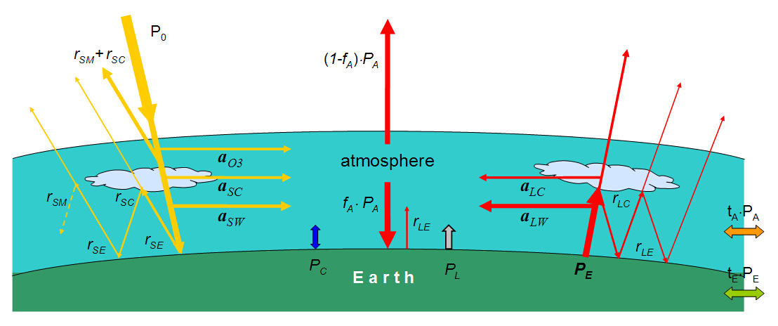
Figure 9. Two-layer climate model of the Earth's surface and atmosphere.
atmosphere as a second, wider layer (see Figure 9), both acting as absorbers and Planck radiators. In
this aspect it is similar to the Dines or Liou models [2224], however, with a lot more features, e.g., the
sw and lw absorptivities, caused by the varying gas concentrations or temperature, and also including
cloud effects for the sw- and lw-radiation, sensible and latent heat transfer as well as all relevant feedback
effects like water vapour, lapse rate, albedo, cloud cover, convection and evaporation.
In equilibrium the surface and atmosphere each donate as much power as they accept from the sun, the
neighbouring layer or a conterminal climate zone.
4.1 Short-Wave Radiation Budget
The solar power irradiating one of these climate zones (tropics, mid-latitudes or high-latitudes) is:
P0 = ES ˇ AZpro
(23)
with AZpro as the projection area perpendicular to the incident light and ES as the solar constant. Then, the
power absorbed by O3 over the stratosphere and tropopause and mostly released as heat in the atmosphere,
may be
1. to atmos:
aO3 ˇ P0
(24)
where aO3 is the integral absorptivity of the O3 molecules.
On its further way through the atmosphere the non-absorbed portion (1-aO3) ˇ Po will partially be
backscattered to space, for which two cases have to be distinguished. Under clear sky conditions primarily
Rayleigh and Mie scattering by molecules and micro-sized particles in the atmosphere will be observed.
This process may be characterized by a scattering coefficient rSM for sun light or sw radiation (although
physically not correct, often designated as reflection). With cloud overcast additional scattering occurs
with an increased scattering coefficient rSA, which may be expressed as sum of the molecular and an
additional cloud scattering contribution rSC with rSA = rSM + rSC, and which is weighted with the cloud
cover CC. Then the total sun light scattered back to space is:
19

OPEN JOURNAL OF ATMOSPHERIC AND CLIMATE CHANGE
1. to space:
((1 -CC)rSM +CCrSA) ˇ (1 - aO3)P0 = (rSM +CC ˇ rSC) ˇ (1 - aO3) ˇ P0
(25)
Radiation propagating through clouds not only suffers from stronger scattering losses but also from an
additional absorption over the cloud path. With a cloud absorptivity aSC the spare power which is released
as heat energy in the atmosphere becomes
2. to atmos:
aSCCC(1 - rSA) ˇ (1 - aO3)P0
(26)
The down-welling radiation also consists of two parts, one representing the clear sky conditions with
weight (1 - CC), the other the cloud covered portion with weight CC. On its further path to the surface
additional absorption losses due to water vapour, CO2 and CH4 show up, which for simplicity are assumed
to occur primarily in the lower troposphere. With an absorptivity aSW we find for the power, transferred
to the atmosphere:
3. to atmos:
aSW [(1 -CC)(1 - rSM) +CC(1 - rSA)(1 - aSC)] ˇ (1 - aO3)P0
(27)
As a first contribution, which can be coupled to the surface layer, it is left:
1. to Earth:
(1 - rSE )(1 - aSW ) [(1 -CC)(1 - rSM) +CC(1 - rSA)(1 - aSC)] ˇ (1 - aO3)P0
(28)
where rSE is the reflectivity of the Earth's surface for sw radiation.
The reflected radiation from the surface not only disappears to space but can again be scatted at the
atmosphere as molecular and cloud scattering, and can also further be absorbed in the clouds. The
reflected power at the surface is
rSE ˇ (1 - aSW ) [(1 -CC)(1 - rSM) +CC(1 - rSA)(1 - aSC)] ˇ (1 - aO3)P0 = rSE ˇ PS
(29)
with the abbreviation PS for Power at the Surface. An additional absorption of this outgoing radiation by
water vapour and CO2 can well be neglected due to saturation effects and bleaching of the radiation on
the stronger absorption bands. But radiation passing again the clouds delivers a second contribution to the
atmosphere:
4. to atmos:
CC(1 - rSA) aSC ˇ rSE PS
(30)
and the amount passing to space is:
2. to space:
((1 -CC)(1 - rSM) +CC(1 - rSA) (1 - aSC)) ˇ rSE PS
(31)
That part, again scattered down and coupled into the surface, is
2. to Earth:
(1 - rSE ) ((1 -CC)rSM) +CCrSA)) rSE ˇ PS
(32)
20

Advanced Two-Layer Climate Model for the Assessment of Global Warming by CO2
After a second reflection at the surface we find the contributions:
5. to atmos:
CC(1 - rSA) aSC ˇ rSE ((1 -CC)rSM +CCrSA) ˇ rSE PS
(33)
3. to space:
((1 -CC)(1 - rSM) +CC(1 - rSA) (1 - aSC)) ˇ rSE ((1 -CC)rSM +CCrSA) ˇ rSE PS
(34)
3. to Earth:
(1 - rSE ) ˇ r2 ((
SE
1 -CC)rSM) +CCrSA))2 ˇ PS
(35)
A third reflection at the surface gives:
6. to atmos:
CC(1 - rSA) aSC ˇ r2 ((
SE
1 -CC)rSM +CCrSA)2 ˇ rSE PS
(36)
4. to space:
((1 -CC)(1 - rSM) +CC(1 - rSA) (1 - aSC)) ˇ r2 ((
SE
1 -CC)rSM +CCrSA)2 ˇ rSE PS
(37)
4. to Earth:
(1 - rSE ) ˇ r3 ((
SE
1 -CC)rSM) +CCrSA))3 ˇ PS
(38)
It is easy to be seen that additional reflections contribute to three power series which under typical
conditions rapidly converge and can be represented by their sum formulas. So, listing up the individual
contributions for the atmosphere, the Earth and space this gives:
atmos:
aO3 + aSCCC(1 - rSA)(1 - aO3) + aSW + rSE aSCCC(1-rSA)(1-aSW ) ×
P
1-r
SA =
SE ((1-CC )rSM +CC rSA)
P0
(39)
[(1 -CC)(1 - rSM) +CC(1 - rSA)(1 - aSC)] ˇ (1 - aO3)
Earth:
[(1 -CC)(1 - rSM) +CC(1 - rSA)(1 - aSC)]
PSE = (1 - rSE )(1 - aSW ) ˇ
ˇ (1 - aO3) ˇ P0
(40)
1 - rSE ((1 -CC)rSM +CCrSA)
space:
[(1 -CC)(1 - rSM) +CC(1 - rSA)(1 - aSC)]2
PSSp =
rSM +CCrSC + rSE ˇ
ˇ (1 - aSW ) ×(1-aO3)ˇP0
1 - rSE ((1 -CC)rSM +CCrSA)
(41)
21

OPEN JOURNAL OF ATMOSPHERIC AND CLIMATE CHANGE
4.2 Long-Wave Radiation Budget
Most of the energy transfer between the two layers occurs through lw radiation, since both the surface
and the atmosphere act as absorbers and Planckian radiators in the mid-infrared (IR). The power PE
emitted by the surface, is absorbed over wider spectral regions by water vapour, CO2 and CH4 within the
lower troposphere, and an additional fraction of 1.5 % by O3 in the stratosphere. With an absorptivity
aLW for the lw radiation the amount
1. to atmos:
aLW ˇ PE
(42)
is absorbed and released in the atmosphere, whereas the non-absorbed fraction can directly escape to deep
space (Rayleigh scattering in the IR is negligible) or is partially backscattered by clouds to the surface. At
a cloud cover CC and a cloud scattering coefficient rLC for lw radiation then the fraction
1. to Earth:
(1 - rLE )CCrLC(1 - aLW ) ˇ PE
(43)
is coupled back to the surface, where rLE represents the reflectivity of lw radiation at the surface.
That portion which is not backscattered but penetrates into clouds, again splits into a stronger absorptive
contribution and a smaller residuum escaping to space. Denoting the cloud absorptivity for lw radiation as
aLC, the power absorbed by the clouds and further transferred to the atmosphere is:
2. to atmos:
CC(1 - rLC)aLC(1 - aLW ) ˇ PE
(44)
With (44) we assume that the absorbed radiation is totally released as internal energy or heat in the
atmosphere due to dominating heat conduction and convection processes. A slightly modified picture
would be that the absorbed power is re-radiated by the clouds, and because of the continuous broad Planck
spectrum only part of this radiation is reabsorbed by the GH-gases in the atmosphere, whereas from the
non-resonant fraction one half goes to space, the other half is rejected down to the surface. However, a
detailed comparison shows that both pictures almost give identical results in the energy balance, and since
the reality might be somewhere between, here we restrict our further discussion on the first assumption.
The power disappearing to space consists of that portion propagating through clear sky areas, and a rest
having transmitted the clouds:
1. to space:
((1 -CC) +CC(1 - rLC)(1 - aLC)) ˇ (1 - aLW ) ˇ PE
(45)
That radiation, backscattered (1st time) from clouds and then reflected at the ground, is again split into
the three parts:
3. to atmos:
C2
C rLE rLC (1 - rLC )aLC (1 - aLW ) ˇ PE
(46)
2. to Earth:
C2
C r2
LC rLE (1 - rLE )(1 - aLW ) ˇ PE
(47)
2. to space:
CCrLCrLE ˇ ((1 -CC) +CC(1 - rLC)(1 - aLC)) ˇ (1 - aLW ) ˇ PE
(48)
22

Advanced Two-Layer Climate Model for the Assessment of Global Warming by CO2
A next round trip delivers the contributions:
4. to atmos:
C3
(
C r2
LE r2
LC 1 - rLC )aLC (1 - aLW ) ˇ PE
(49)
3. to Earth:
C3
(
C r3
LC r2
LE 1 - rLE )(1 - aLW ) ˇ PE
(50)
3. to space:
C2
ˇ ((
C r2
LC r2
LE
1 -CC) +CC(1 - rLC)(1 - aLC)) ˇ (1 - aLW ) ˇ PE
(51)
Including further reflections and scattering events leads again to respective power series for the two
layers and the space. Summing up all these contributions and taking into account the initial radiation loss
PE from the Earth's surface we find:
atmos:
C
P
C
EA =
aLW +
(1 - rLC)aLC(1 - aLW ) ˇ PE
(52)
1 -C r
r
C LE LC
Earth:
C r
P
C LC
EE = -
1 -
(1 - rLE )(1 - aLW ) ˇ PE
(53)
1 -C r
r
C LE LC
space:
1
PESp =
[(1 -CC) +CC(1 - rLC)(1 - aLC)] ˇ (1 - aLW ) ˇ PE
(54)
1 -C r
r
C LE LC
The atmosphere also represents a Planckian radiator, which emits the power PA. Due to the temperature
distribution over altitude a smaller fraction (1 - fA) 39 % of this lw radiation escapes to space (see (22),
the other part fA 61% is directed downward. At the surface some smaller fraction of the down-welling
radiation is reflected back and remains in the atmosphere, whereas the main part is absorbed by the surface.
This supplements the lw radiation balance for the two layers and the space, for which we find:
atmos:
PAA = - ((1 - fA) + fA - rLE fA) ˇ PA = -(1 - rLE fA) ˇ PA
(55)
Earth:
PAE = (1 - rLE ) fA ˇ PA
(56)
space:
PASp = (1 - fA) ˇ PA
(57)
4.3 Sensible and Latent Heat
Most of the energy transfer between the surface and atmosphere occurs by lw absorption and emission
processes. However, additional energy can be transferred through sensible and latent heat. While sensible
heat represents the energy transfer through thermal conduction and convection from the warmer to the
colder layer, latent heat describes the energy transfer resulting from phase transitions of evaporating water
23

OPEN JOURNAL OF ATMOSPHERIC AND CLIMATE CHANGE
or sublimating ice at the surface and subsequent release of the vaporization energy in the atmosphere,
when the water vapour condenses and falls back as precipitation.
Therefore, the total energy balance between the surface and atmosphere has to be supplemented by the
heat transfer between both layers.
The driving force for thermal conduction and convection is the temperature difference at the boundary
layer between surface and atmosphere. In addition, advection in form of a horizontal energy transfer along
the boundary through wind and water currents takes place. This transfer is only indirectly dependent
on the temperature difference, therefore, it is close-by to assume a power transfer through sensible heat,
represented by a temperature independent portion PC0 and a temperature dependent part in the form:
PC = PC0 + hCAZ(TE - TAC)
(58)
with hC as the heat transfer coefficient, AZ as the surface area of a climate zone, TE as the Earth's surface
temperature and TAC as the air temperature at the convection zone.
An energy transfer from the surface to the atmosphere through latent heat is directly affected by
the temperature TE of the surface, since with increasing temperature more water is evaporating and
more precipitation expected. Generally latent heat just represents the difference in enthalpy for the
transformation between two phases of consideration, and according to Kirchhoff's equation (see, e.g. [6],
p.123), changes in latent heat are directly proportional to temperature changes with a proportionality
factor, given by the difference of the specific heats in the two phases. To allow some smaller deviations
from this general response over a wider temperature interval, and on the other hand to express only
changes in latent heat around a point of reference - this is of particular interest for our considerations here
- we assume a similar relationship for latent heat as applied for sensible heat:
PL = PL0 + lH AZ(TE - T0)
(59)
with PL0 as a fixed contribution defining the point of reference, T0 as the freezing temperature, and lH as
the respective heat coefficient.
For an energy budget, which is restricted to a specific climate zone, an additional exchange between
these zones through atmospheric and oceanic currents has to be included. The power transfers PTA in
the atmosphere and PTE along the Earth's surface to or from an adjacent zone are governed by energy
differences and heat fluxes between the zones. Since any changes in the energy budget also retroact on
the transfer between two zones and such changes are directly reflected by the radiated powers, the transfer
between adjacent zones may be expressed in units of PA and PE . Then, with an increasing or decreasing
balance in one zone in first order also the flux to or from a neighbouring region is changing as:
PTA = tA ˇ PA resp. PTE = tE ˇ PE
(60)
with tA and tE as transfer factors for the atmospheric and terrestrial heat transfer. They are negative, when
the net flux from a considered zone goes out, and they are positive, when power is sucked up.
4.4 Total Radiation and Energy Budget
At thermal equilibrium the absorbed solar radiation must be balanced by the net emission of lw radiation
of EASy to space. This is conservation of energy and the demand of the first law of thermodynamics.
24

Advanced Two-Layer Climate Model for the Assessment of Global Warming by CO2
A balance for each layer, and complementarily for space, gives a coupled equation system describing
the mutual interdependence of the power fluxes between the layers and space.
For the atmosphere we sum up the in- and outgoing fluxes listed in equations (39), (52), (55) and
(58)-(60), for the Earth those listed in (40), (53), (56), (60) and (58)-(59) with opposite sign, and for the
space the radiation terms of (41), (54) and (57), which just must balance the incident solar power:
Atmosphere:
PSA + PAA + PEA + PC + PL + PTA = 0
(61)
Earth:
PSE + PAE + PEE - PC - PL + PTE = 0
(62)
Space:
PSSp + PASp + PESp
= P0
(63)
To identify the mutual coupling of PE and PA, in more elaborate form these equations can be written as:
Atmosphere:
PSA - PA + A PE + PC + PL = 0
(64)
Earth:
PSE + PA - B PE - PC - PL = 0
(65)
Space:
PSSp + PA +C PE
= P0
(66)
with the abbreviations:
= 1 - rLE fA - tA
= (1 - rLE ) fA
= 1 - fA
(67)
CC
A = aLW +
(1 - rLC) aLC(1 - aLW )
(68)
1 -C r
r
C LE LC
C r
B = 1 - t
C LC
E -
(1 - rLE ) (1 - aLW )
(69)
1 -C r
r
C LE LC
1
C =
[(1 -CC) +CC(1 - rLC)(1 - aLC)] ˇ (1 - aLW )
(70)
1 -C r
r
C LE LC
The upper equation system is over-determined, since one relation, e.g., the balance for space is already
implicitly a consequence of the other two relations and only expresses right away the conservation of
radiation energy at the TOA. Thus, for a further elucidation of an adjusting equilibrium between the layers
only two of these equations are of relevance. Here we further rely on the upper two equations (64) and
(65).
In the special case of known sensible and latent heat, the remaining balance equations can easily be
solved yielding:
25

OPEN JOURNAL OF ATMOSPHERIC AND CLIMATE CHANGE
PSE + PSA - ( - )(PC + PL)
PE =
(71)
B - A
1
PSE + PSA - ( - )(PC + PL)
PA =
PSA + PC + PL + A ˇ
.
(72)

B - A
In general, however, PC and PL are no fixed quantities, but at least to some degree are directly influenced
by the energy balance between the layers and therewith by the respective temperatures TE and TA (see
(58)-(59)).
When the Earth and the atmosphere are considered as black- or grey-body radiators, emitting the
radiation power PE at an average surface temperature TE and the power PA at a mean atmospheric
temperature TA, the Stefan-Boltzmann law [5, 6] provides a well-known relationship between the radiated
power and the temperature. For the Earth's surface as a Planckian radiator this gives:
PE = E ˇ ˇ AZ ˇ T 4
E
(73)
with the emissivity E of the surface and the Stefan-Boltzmann constant = 5.67ˇ10-8W /m2/K4.
To characterize also the atmosphere by an average temperature according to Stefan-Boltzmann, we
have to have in mind, that due to the asymmetric radiation of the atmosphere, a fraction fA is emitted
downward and (1 - fA) upward. As a consequence we have to distinguish between two mean temperatures
TA,l and TA,u characterizing the lower and the upper troposphere, and defined by the relations:
fA ˇ PA = A ˇ ˇ AZ ˇ T 4
A,l
(74)
(1 - fA) ˇ PA = A ˇ ˇ AZ ˇ T 4
A,u
(75)
Whereas (75) is not further needed for the succeeding discussion, (74) is relevant to embrace any
feedback of the convection to the total balance. Since TA,l typically reflects a temperature, equivalent to an
air layer temperature in about 800m altitude, but convection is only dominant over about 200m height, the
temperature difference (TE - TAC) in (58) is assumed to be just one quarter of the difference (TE - TA,l).
For simplicity we write for the lower tropospheric temperature only TA. So, for the further considerations
(58) may be replaced by
PC = PC0 + 1/4hCAZ(TE - TA)
(76)
The relations (73) and (74) then represent a link between the balance equations (64)-(65) on the one
hand side and the sensible and latent heat ((76) and (59)) on the other side. Together all these relations
form a nonlinear equation system, in which the radiation and heat fluxes are coupled to each other via the
temperatures TE and TA.
This equation-system can be solved iteratively. With initial conditions PC = PC0 and PL = PL0, in a first
step initial values for PE and PA are calculated by means of the balance equations, and with (73)-(74) initial
values for the temperatures TE and TA are derived. According to (76) and (59) with these temperatures
first improved values for PC and PL are found, which in a next iteration step are inserted in (64)-(65) to
find new powers and temperatures. This procedure is repeated till the calculations show self-consistency.
To evaluate the influence of CO2 on global warming and by this to determine the CO2 climate
sensitivity, this kind of calculation has to be performed at different CO2 concentrations, at least at the
26

Advanced Two-Layer Climate Model for the Assessment of Global Warming by CO2
actual concentration as a reference and, e.g., the doubled concentration. Due to the changing sw and
lw absorptivities at these different concentrations also the radiation and energy balance will be altered
and therewith the temperatures. Since any deviation from the reference temperature causes a chain of
additional feedback processes, in a second loop these feedbacks are included and the calculations are
consecutively repeated until also with these corrections self-consistency for the temperature values is
found.
5. SIMULATIONS WITHOUT SOLAR INFLUENCE
The sw and lw absorptivities were calculated for global conditions as well as for the three climate
zones. Therefore, also individual simulations for each climate zone could easily be performed. However,
comparison with radiation and energy budget data for theses zones are quite restricted. So, here we
only consider simulations for the global Earth-atmosphere system. Nevertheless the separate spectral
calculations are important, to derive from these data the water vapour and lapse rate feedback as outlined
in section 3. In this section only simulations of global warming, caused by CO2 alone will be presented.
The additional influence of solar variations will be discussed in section 6.
5.1 Adaptation to Satellite Measurements
For our simulations we use parameter values as listed in Table 5. The sw and lw absorptivities result
from the calculations presented in section 2 and are valid for standard atmospheric conditions with a mean
water vapour concentration at ground of 1.46 %, a CO2 concentration of 380 ppm, a CH4 concentration of
1.8 ppm and a varying O3 concentration over the stratosphere with a maximum around 38 km altitude.
The average cloud cover with CC = 66% was adopted from published data of the International Satellite
Cloud Climatology Project (ISCCP) [25]. The other parameters like cloud and sw ozone absorptivities,
the scattering coefficients at clouds and the atmosphere as well as the Earth's reflectivities were adapted
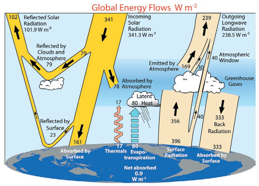
in such a way that all radiation and heat fluxes almost exactly reproduce the widely accepted radiation
and energy budget scheme of Tremberth, Fasullo and Kiehl [20] (hereafter TFK-scheme, see Figure
10), which essentially relies on data from satellite measurements within the ERBE and CERES program
[1519]. So, this adaptation quasi yields a calibration of our model to the observed up- and down-welling
fluxes under standard conditions in the atmosphere and for constant heat fluxes between the surface and
atmosphere.
A quite important parameter for reproducing the TFK-scheme is the asymmetry factor fA, which
specifies the amount of downward directed lw radiation in comparison to the totally emitted power of the
atmosphere. Therefore, it directly determines the lw fluxes in up- and downward direction, and by this
controls the lw radiation balance. Its size sensitively depends on the lapse rate and the ground temperature,
but also on the water vapour content and the diffusivity factor. From our radiation transfer calculations
(see section 3) we find variations from 57.6 - 62.6 % over the climate zones and an averaged value of fA =
61.0 %. We achieve good consistency with the TFK-data for fA = 61.8 %, therefore, this value will be
used in the further computations.
Comparison of our simulations with the TFK-scheme (see Table 6) then shows quite good agreement
to each other and by this confirms the basically correct and reliable operation of the presented model.
27

OPEN JOURNAL OF ATMOSPHERIC AND CLIMATE CHANGE
Table 5. Parameters for adaptation to the TFK-data.
parameter
symbol
unit
value
total solar irradiance - TSI
Es
W /m2
1365.2
averaged solar flux
IS,av
W /m2
341.3
Earth's surface area
AE
1012m2
510
projection area
Apro
1012m2
128
Cloud cover
CC
%
66.0
sw molec. scattering coef.
rSM
%
10.65
sw cloud scattering coef.
rSC
%
22.0
sw Earth reflectivity
rSE
%
17.0
sw absorptivity: ozone
aO3
%
8.0
sw cloud absorptivity
aSC
%
12.39
sw absorptivity: H2O-CO2-CH4
aSW
%
14.51
lw cloud scattering coef.
rLC
%
19.5
lw Earth reflectivity
rLE
%
0.0
lw cloud absorptivity
aLC
%
62.2
lw absorpt.: H2O-CO2-CH4-O3
aLW
%
82.58
Earth emissivity
E = 1 - rLE
%
100.0
atmosph. emissivity
A
%
87.5
asymmetry factor
fA
%
61.8
sensible heat flux
PC/AE
W /m2
17.0
latent heat flux
PL/AE
W /m2
80.0
Figure 10. Radiation and Energy Budget of the Earth-atmosphere system (after Tremberth, Fasullo and Kiehl [20],
reproduced with permission of the authors).
A smaller systematic deviation, however, results from the fact that the up- and down-welling fluxes
in the TFK-scheme are not completely balanced, but contribute to a net surface absorption of 0.9W /m2.
Therefore, the total outgoing radiation, in our data 239.4 W /m2, is by this amount larger, and a similar
discrepancy with opposite sign appears for the back-radiation with some smaller feedback also on the
fA-factor.
It should also be noticed, that Tremberth et al. use a terrestrial radiation flux, which corresponds to
a global mean temperature of 16 ° C instead of the generally applied 15 ° C. This discrepancy can be
28

Advanced Two-Layer Climate Model for the Assessment of Global Warming by CO2
Table 6. Calculated radiation fluxes and comparison with the TFK-data.
flux (W/m2)
this model
TFK-data
sw: incoming solar radiation
341.3
341.3
backscattered from molecules
11.4
backscattered from clouds
67.6
together backscattered
79.0
79
reflected at Earth's surface
22.9
23
total reflected solar radiation
101.9
101.9
absorbed by O3,
27.3
clouds,
19.1
water vap, CO2, CH4
31.6
total absorption atmosphere
78.0
78.0
absorption in surface
161.3
161
lw: surface radiation
396.4
396
absorbed by GH-gases
322.4
absorbed by clouds
24.4
backscattered by clouds
9.5
absorb. & scat. surface radiation
356.3
356
sensible heat
17.0
17
latent heat
80.0
80
total absorption in atmosph.
521.8
outgoing radiation fr. atmosph.
199.4
199
outgoing directly from surface
40.0
40
total outgoing radiation
239.4
238.5
backradiation
332.0
333
net emission of surface
64.4
total outgoing radiation at TOA
341.3
340.4
explained by different averaging procedures applied to derive a global mean and from this to calculate the
radiated power by the Stefan-Boltzmann law.
Somewhat surprising is, that they assume a reflectivity for lw radiation at the surface of rLE = 0 and
therefore an emissivity E = 1 - rLE = 1, although it is mentioned in their paper that the Earth is no ideal
blackbody radiator and in some areas the reflectivity is at least several %. To maintain the otherwise good
conformity to the TFK-scheme, in this frame we assume also a zero Earth reflectivity for lw radiation and
use a ground temperature of 16 ° C.
Since the objective of our further investigations is to evaluate the influence of CO2 on global warming,
we use the specified parameters in Table 5 as reference marks, which in some sense define a working
point for the further considerations, in particular they determine the reference temperature of the Earth's
surface at a CO2 concentration of 380 ppm. Only deviations from this reference, caused by a changing
CO2 concentration and the different feedback processes, are of further interest, not so much absolute
temperature levels.
5.2 Influence of some Model-Parameters on the Balance
In order to assign the influence and importance of the different parameters, it seems worthwhile first to
discover the response of the global system to any changes of these parameters. This is a prerequisite for a
better understanding and interpretation of the complex heating and cooling effects which partially amplify
but also erase each other.
There is no doubt that the sw and lw absorptivities of the GH-gases have a dominant influence on
29

OPEN JOURNAL OF ATMOSPHERIC AND CLIMATE CHANGE
any balance between the two layers. This will be discussed in more detail in the next subsection.
But also the cloudiness, characterized by the key parameter cloud cover CC as well as the sw and lw
scattering coefficients and absorptivities have a significant affect on this balance, and this even in a
somewhat ambiguous way. While a reduced cloud cover generally causes surface heating due to the higher
transmissivity of the atmosphere for solar radiation, at the same time this also increases the transparency
for the outgoing lw radiation from the surface to space and therefore contributes to a stronger cooling. So,
to some degree both effects can compensate each other, depending on the actual weather conditions, the
day time, or in our simulations depending on the choice of the scattering and absorption parameters.
The rejected solar radiation at the atmosphere and clouds with 79 W /m2 can easily be adjusted by one
or both sw scattering coefficients, which together determine the total backscattered flux according to (25):
((1 -CC)rSM +CCrSA) ˇ (1 - aO3)P0 = (rSM +CC ˇ rSC) ˇ (1 - aO3) ˇ P0
(25)
with rSA = rSM + rSC. However, the response of EASy to any changes in the cloud cover additionally
depends on the weighting of rSC in comparison to rSM , and also on the size of the lw cloud scattering rLC.
In our simulations these parameters are adjusted in such a way, that on the one hand side the fluxes
agree with the TFK-data, on the other side they reproduce the observations of the global mean temperature
change with cloud cover. From the ISCCP-data [25] it is found that 1 % of a reduced cloud cover causes a
temperature increase of about 0.06 - 0.07 ° C. This tendency is also confirmed by data of Hartmann [26],
well knowing that such observations are superimposed by several other effects influencing the temperature
data. With the parameter set in Table 5 we can well reproduce this temperature response to the cloud
cover with a global mean temperature of 19.8 ° C at CC = 0 % and 13.0 ° C at 100% overcast.
The cloud absorptivities and surface reflectivities are not very sensitive parameters with respect to
consequences on the climate sensitivity, but their correct choice insures the right adaptation of the total
atmospheric and surface absorptions. In this sense they define the reference temperatures at which the
two layers are found in equilibrium.
It should be noticed that the sw and lw cloud and ground absorptions are generally the result of multiple
up and down scattering events, at least as long as the reflections at the surface are not zero. Therefore,
the listed fluxes and absorptions in Table 6 cannot simply be derived by multiplying the incident or
outgoing radiation with the respective absorptivity or reflectivity, but have to be calculated using some of
the relations considered in subsections 4.1 or 4.2, e.g., the sw reflection at the surface with 22.9 W /m2 is
not only a function of the ground reflectivity with rSE = 17 % but is additionally influenced by several
other parameters (see also (41)):
rSE (1 - aSW ) ˇ (1 - aO3)
ES
IR = ((1 -CC) ˇ (1 - rSM) +CC(1 - rSA) ˇ (1 - aSC))2 ˇ
ˇ
(77)
1 - rSE CCrSA + (1 -C
4
C))rSM
So, an effective reflectivity, related to the incident solar flux at TOA, is only 22.9/341.3ˇ100 = 6.7 %, or
with respect to the primary flux (before the first reflection at surface) is 22.9/186.1ˇ100 = 12.3 %.
While the surface emissivity E has a direct influence on the lw radiation budget, but was set to unity
to agree with the TFK-scheme, the atmospheric emissivity A in our model is only needed to calculate
the mean temperature of the lower troposphere, which affects the temperature dependent part of thermal
convection between the layers (see (76)) and insofar also causes a direct feedback on the adjusting balance.
Generally the atmospheric emissivity is identical to the total lw absorptivity as given by (68) with:
CC
A = A = aLW +
(1 - rLC) aLC(1 - aLW )
(78)
1 -C r
r
C LE LC
30

Advanced Two-Layer Climate Model for the Assessment of Global Warming by CO2
and, therefore, consists of the absorption caused by GH-gases as well as of the cloud absorption. Since
aLW is varying with the CO2 concentration, also A becomes a function of this concentration, but owing
to the second term in (78) on a slightly varying background. This is in so far of some importance, since
an atmospheric temperature, calculated from the balance equations with the emissivity of (78), shows a
significantly lower sensitivity to concentration variations than assuming a constant emissivity, as this is
generally applied. As a direct consequence the sensible heat flux increases with the CO2 concentration
and causes additional cooling of the surface, thus leading to a negative feedback in the EASy-balance.
5.3 Direct Influence of CO2 on the Surface-Temperature
GH-gases have a twofold influence on the EASy energy and radiation budget. While they attenuate
the solar radiation and by this the amount which can be absorbed by the surface, they block a great deal
of the terrestrial radiation to be directly rejected to space and thus, cumber the energy loss to space. In
Table 2 and Table 3 are compiled the integral sw and lw absorptivities of the well-mixed GH-gases water
vapour, CO2, CH4 and O3 . They were derived from line-by-line calculations and determined for different
CO2 concentrations from 0-770 ppm. To assess the influence of CO2 on global warming, we use these
absorptivities and calculate for each pair of sw and lw absorptivities at otherwise identical conditions
the respective surface and atmospheric temperature. For the case of clear sky (CC = 0) this is shown in
Figure 11.a. The red graph indicates the Earth's temperature TE and the blue graph the lower tropospheric
temperature TA. The increase of TE at doubled CO2 concentration (from 380 to 760 ppm) defines the CO2
climate sensitivity as a measure for the response of EASy on a changing CO2 concentration. In this case, at
clear sky conditions and without any feedback effects, we find a climate sensitivity of CS = 1.11 ° C which
is in surprisingly good agreement with the IPCC value also of CS = 1.1 ° C (without feedback processes,
but generally assuming mean cloud cover) and based on the RF- concept [2, 3]. Additionally shown is a
logarithmic plot (green graph), indicating that due to saturation effects and only far wing absorption at
higher CO2 concentrations the surface temperature can well be approximated by a logarithmic function.
From Figure 11.a we also see that the lower atmosphere responds less sensitively to the CO2 changes.
The respective temperature increase of TA at doubled CO2, which we may call here as air sensitivity, is
only AS = 0.45 ° C and significantly smaller than the climate sensitivity. This lower response is explained
by the fact that with increasing CO2 concentration also the emissivity of the atmosphere is increasing (see
(78)) and so compensating to some degree the higher absorption in the atmosphere.
The dominant influence of clouds on the whole energy budget can be seen from Figure 11.b. When
repeating the same calculation as before, only choosing the mean cloud cover of 66 %, not only the
temperatures are considerably dropping (TE by 3.8 ° C, TA by 2.8 ° C), but also the climate and air
sensitivities are significantly reducing to CS = 0.55 ° C and AS = 0.19 ° C.
While the falling temperatures are a consequence of the dominating shielding effect for solar radiation
(in the real climate system particularly caused by the lower clouds), the smaller sensitivities are a direct
consequence of the increasing influence of the lw cloud absorption and backscattering, by which the
importance of the GH-gases is more and more repelled. So, at 100 % cloud cover the air sensitivity would
completely disappear and the climate sensitivity be reduced to 0.2 ° C.
31

OPEN JOURNAL OF ATMOSPHERIC AND CLIMATE CHANGE
Figure 11. Calculated Earth-temperature TE (red) and lower tropospheric temperature TA (blue) as a function of the
CO2 concentration under a) clear sky, b) 66% cloud cover. Logarithmic approximation - green.
5.4 Feedback Processes
Most of the climate scientists agree, that an increasing absorption with rising CO2 concentration alone,
as discussed in the previous subsection, would only moderately contribute to any global warming. The
greater worry, however, is that already smaller perturbations, as caused by the GH-effect, may initiate
further side effects, which could significantly amplify the primary perturbation and even result in a total
destabilization of the quasi equilibrium conditions of EASy. These side-effects are known as feedback
processes, which on one side can amplify an initial deviation (positive feedback) or on the other side can
also attenuate this deviation (negative feedback).
5.4.1 Water-Vapour-Feedback
Due to the Clausius-Clapeyron-equation the water vapour content in air is rapidly increasing with rising
temperatures. Therefore, also the water vapour absorption is further increasing and generally contributes
to a positive feedback in the total budget. In the literature this feedback is designated as the most serious
effect with dramatic amplification values of 1.5 - 3 [27].
Our own investigations, however, show a less dramatic influence of water vapour. One aspect is that,
32

Advanced Two-Layer Climate Model for the Assessment of Global Warming by CO2
similar to CO2, also the water lines are already strongly saturating over wider spectral regions. Therefore,
with increasing vapour concentration only the far wings of these lines and weak absorption bands can
further contribute to an additional absorption, which roughly logarithmically increases with the vapour
concentration.
In this context, obviously some physical misinterpretation of the absorption behaviour of a gas exists,
see e.g. Ref. 27. So, it is concluded that not the absolute change in the water vapour concentration,
but its fractional change would govern the strength as a feedback mechanism; and from this statement
it is deduced, that the largest contribution to the feedback occurs in the upper troposphere. However,
molecules can only absorb radiation, which is still available on the absorption frequencies. Since the
lower atmospheric layers with the strongly pressure broadened spectral lines already filter the outgoing
radiation up to the far wings and by this determine the logarithmic absorption behaviour, there is no
further radiation left for the narrower lines in the upper troposphere, only from adjacent layers of the
atmosphere itself. In addition, the absorption strength on the line centre, and thus the saturation behaviour
for the radiation, is almost the same in the upper troposphere as in the lower troposphere, since with
reducing pressure and temperature on the one hand the number of molecules decreases, but due to the
reducing linewidth the linestrength increases. This is the law of spectral stability.
Another aspect is that always both, the sw and lw absorptions have to be considered. While the lw
outgoing radiation is more efficiently blocked and so contributes to positive feedback, the sw radiation is
also stronger absorbed in the atmosphere, but less of it reaches the surface and therefore supplies a net
negative feedback.
Our calculations for the sw and lw absorptivities in section 2 were performed for three climate zones,
which differ in their mean humidity and ground temperature. Figure 12 shows the absorptivities in these
zones as a function of the respective ground temperatures at 380 ppm CO2.
Figure 12. Calculated sw absorptivity (blue) and lw absorptivity (red) for the three climate zones plotted as a func-
tion of the respective zone temperatures.
Since the water content in each climate zone was derived from actual GPS-measurements [10] and
this water content used to calculate the water vapour concentration at this zone-temperature, the graphs
in Figure 12 directly reflect the temperature dependence of the water vapour concentration on the
absorptivities. The linear increase is the result of an exponential growth of the water vapour concentration
with temperature due to Clausius-Clapeyron and on the other hand a logarithmic rise of the absorptivity
33

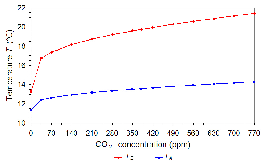
OPEN JOURNAL OF ATMOSPHERIC AND CLIMATE CHANGE
with the vapour concentration due to saturation effects.
The sw and lw absorptivities can well be represented by straight lines with the slopes
daSW /dTE = 0.097 %/C
(79)
and
daLW /dTE = 0.38 %/C
(80)
With these parameters the water vapour feedback can be included in the further considerations by
an iterative procedure, as already outlined in section 4. In a first step the temperature deviation from
the reference temperature TR, caused by a deviation of CO2 from the reference concentration (here 380
ppm) is calculated. This T -offset is used to compute with the feedback parameters the corrections in
the absorptivities. With the new values again corrected temperatures are determined, which give new
absorption corrections. This is repeated, until the temperatures show self-consistency.
The result of such calculation is illustrated in Figure 13, representing the temperature increase of TE
and TA with water vapour feedback at clear sky conditions. The respective climate sensitivity increases
from CS = 1.11 ° C to 1.66 ° C and the air sensitivity from AS =0.45 to 0.71 ° C, giving an amplification
factor, caused by water vapour feedback, for CS of 1.5 and for AS of 1.58.
At regular cloud cover of 66 %, however, CS only increases from 0.55 ° C to 0.65 ° C and AS from
0.19 ° C to 0.23 ° C corresponding to reinforcements of 1.19 and 1.22.
Figure 13. Calculated surface temperature TE (red) and lower tropospheric temperature TA (blue) as a function of
CO2 concentration with water vapour feedback at clear sky.
5.4.2 Lapse-Rate-Feedback
Under mean global conditions the average temperature decrease with altitude over the troposphere is
specified as 6.5 ° C/km and is assumed to be constant up to the tropopause at about 11 km altitude [9]. As
34

Advanced Two-Layer Climate Model for the Assessment of Global Warming by CO2
already outlined in section 3 , this lapse rate has a direct influence on the power, which is asymmetrically
re-radiated by the atmosphere in downward and upward direction. From radiation transfer calculations we
find, that at this standard lapse rate the fraction radiated downward is fA = 61.0 %, and that rejected to
space (1 - fA) = 39.0 %, respectively. When this vertical temperature profile changes, it also induces a
climatic effect, known as lapse rate feedback.
Global circulation models predict an enhanced warming in the upper troposphere of tropical regions,
particularly in response to an increasing water vapour concentration. This would result in a negative
feedback. On the other hand, at mid- to high-latitudes, a larger low level warming is expected as response
to the positive radiative warming, thus, providing a positive feedback. Since the influence of the tropics is
assumed to dominate, a resulting negative feedback of -0.8 Wm-2K-1 ( -20 %) is predicted [27, 28].
Independent of these effects we consider an additional slightly different influence of a changing lapse
rate on the climate. It is well-known that the tropopause height is significantly varying from climate zone
to climate zone (also over the seasons) and in so far is directly related to the local ground temperature.
Whereas the mean absorption and re-radiation over a longer or shorter path in the troposphere will not
noticeably be influenced, as long as the optical depth is almost constant, changes of the lapse rate in
these climate zones with the ground temperature directly affect the asymmetry factor fA and thus the total
balance of EASy.
In the literature quite contradictory models can be found about the temperature distribution over the
troposphere. So, one model assumes that due to convection the lapse rate over the troposphere is always
constant and with a changing ground temperature the tropopause height is synchronously shifted up or
down. The other extreme is to expect a constant height, at least within one climate zone, and to suppose
that any ground temperature variations only affect the lapse rate.
From calculations with a fixed tropopause height over all zones and therefore a maximum lapse rate
change from 7.5 ° C/km for the tropics (ground temperature: 26 ° C) to 4.5 ° C/km for the polar region
(temperature: -7 ° C), we derive a temperature dependence of the asymmetry factor of df A/dTE = ba
= 0.145 % / ° C (see subsection 3.3, Figure 8). The reality obviously lies somewhere between these
extremes, and it seems plausible to use a somewhat smaller value. Together with the predicted negative
feedback, determined by the dominating tropical influence, we estimate a temperature dependence of:
d fA = ba = 0.05 %/C
(81)
dTE
For the respective sensitivities we then find CS = 1.22 ° C and AS = 0.6 ° C, which under regular cloud
cover reduce to CS = 0.62 ° C and AS = 0.24 ° C .
Since the water vapour has a more or less stronger influence on the lapse rate, both effects are often
considered together [27]. For the combined water vapour and lapse rate feedback we then get an
amplification factor under clear sky conditions of 1.74 and with clouds of 1.37.
5.4.3 Earth Albedo Feedback
A further feedback results from the fact that with increasing ground temperature the Earth's reflectivity
will be influenced, caused by the ice cover in the polar regions and changes of the vegetation. With
varying reflectivity particularly the sw radiation balance will be modified in such a manner, that with
35

OPEN JOURNAL OF ATMOSPHERIC AND CLIMATE CHANGE
reducing reflectivity more power is absorbed by the Earth's surface which then contributes to an additional
heating of the ground.
This Earth albedo influence is estimated as a positive feedback with an amplification between 10 and
15 % [27, 28]. In our simulations we introduce this albedo feedback as a temperature dependent change
of the Earth's reflectivity with:
drSE = ef = -0.17 %/C
(82)
dTE
which under clear sky contributes to an increase of the climate sensitivity of 15 % and at mean overcast of
12 %.
5.4.4 Convection Feedback
The sensible heat flux at the reference CO2 concentration of 380 ppm and temperature TR = 16 ° C
(for clear sky 19.8 ° C) was chosen to be 17 W /m2 in agreement with the TFK-scheme, and this flux
was assumed to be constant in the previous simulations. From (76), however, we know that the heat
transfer will generally be composed of two contributions, one constant part IC0 = PC0/AZ, determined by
temperature independent processes for the heat transport at the boundary, and a second part, governed by
the temperature difference between the surface and atmosphere with
IC = PC/AZ = IC0 + 1/4hC(TE - TA)
(83)
Due to the second term in this equation any temperature changes induced by CO2, also initiate a
feedback on EASy, which we may call convection feedback.
From Figure 11 and Figure 13 it can well be recognized that the air temperature reacts less sensitively
to concentration variations than the Earth-temperature, and the difference (TE - TA) increases with
increasing CO2 concentration. Therefore, also the sensible heat flux grows with the concentration. Since
an increasing flux from the surface to the atmosphere contributes to an additional cooling, the resulting
feedback will be negative.
The size of this feedback gets maximum, when the first term on the right side of (83) vanishes and
the total heat flux of 17 W /m2 at 380 ppm CO2 is determined by the second term. At clear sky and a
temperature difference of (TE - TA ) = 6.2 ° C then the heat convection coefficient can assume a maximum
value of hC,max = 11 W/m2/ ° C, whereas under regular cloud cover with a temperature difference (TE - TA)
= 5.2 ° C this maximum value is hC,max = 13 W/m2/ ° C. When choosing a smaller convection parameter,
this automatically reduces the feedback but increases the first term in (83), so that at the reference CO2
concentration always a sensible heat flux of 17 W/m2 is guarantied.
For hC = 10 W/m2/ ° C for both cases, uncovered and covered, at clear sky we calculate a climate
sensitivity of CS = 0.96 ° C corresponding to an attenuation of 0.86, and at regular cloud cover CS =
0.45 ° C with a reduction factor of 0.82. Sensible heat in this case consists of a constant contribution of 4
W/m2 and a temperature dependent part of 13 W/m2 at TE = 16 ° C.
36

Advanced Two-Layer Climate Model for the Assessment of Global Warming by CO2
5.4.5 Evaporation Feedback
Similar to convection also evaporation of water and sublimation of ice contribute to cooling of the
surface. Since an increasing Earth temperature further forces these processes, they also result in a negative
feedback, which we call evaporation feedback. As already outlined in section 4, the latent heat flux may
be expressed as:
IL = PL/AZ = IL0 + lH (TE - T0)
(84)
consisting of a temperature independent contribution IL0, and a second term proportional to the ground
temperature above the freezing point (TE - T0). Under regular conditions IL0 almost vanishes, and the
feedback, then only determined by the second term in (84), gets maximum. Since the total flux at the
reference CO2 concentration of 380 ppm is held fixed to 80 W /m2 in agreement with the TFK-scheme,
at mean cloud cover the heat transfer coefficient lH can assume a maximum value of 5 W /m2/ ° C (80
W /m2/16 ° C) and at clear sky 4 W /m2/ ° C (80 W /m2/19.8 ° C). When for some reason the heat transfer
is less sensitively responding to temperature changes (e.g., less rapidly increasing precipitation rate or
saturating evaporation), lH and by this the feedback may further be reduced. Then, in the same way, as
the second term in (84) decreases, the first term increases.
Without clouds and maximum lH = 4 W /m2/ ° C we find a climate sensitivity of CS = 0.72 ° C; at mean
cloud cover and with lH,max = 5 W /m2/ ° C it reduces to CS = 0.3 ° C, which corresponds to an attenuation
by a factor of 0.56. So, latent heat can contribute to significant negative feedback.
In this context it should be noticed that generally evaporation and convection feedbacks are not
mentioned or included in climate models considered by the IPCC, although obviously they have a quite
strong influence on the adjusting temperature levels.
5.4.6 Thermally Induced Cloud Feedback
Comparison of the preceding simulations under clear sky and at cloudiness already demonstrates the
dominant influence of the cloud cover on the self-adjusting equilibrium between the Earth and atmospheric
layers. So, the climate sensitivity drops to about half its value compared to clear sky conditions, and the
ground temperature approximately changes from 20 to 16 ° C, when the cloud cover increases from 0 to
66 %. This temperature response was adopted from the ISCCP-observations of the global warming and
mean cloud cover variations over the period 1983 - 2010 [25].
However, when for some reason the driving force for any of these observed changes is not the cloud
cover but the temperature, acting back on the cloudiness, we have to consider an additional feedback
process, which then further amplifies the GH-effect and even might overcompensate the previously
observed reduction of sensitivities at cloudiness.
It is quite obvious that the registered temperature changes will not exclusively result from cloud
variations or vice versa, but may also be influenced by variations of the solar radiation, the humidity or
internal oscillations. In addition, also observations are known, particularly in the tropics, were just the
opposite trend is found, that with increasing temperature also the cloud cover is increasing [2932], which
then contributes to negative feedback.
Therefore, obviously the worst case will be, to attribute any response of the cloud cover CC, as derived
from the ISCCP-data, only to the surface temperature change TE and to address this change only to the
37

OPEN JOURNAL OF ATMOSPHERIC AND CLIMATE CHANGE
CO2-GH-effect, (CO2 induced cloud feedback), this at least around the mean cloud cover of 66 % and
the mean global temperature of 16 ° C. Since even at very high temperatures clouds will not completely
disappear, we suppose a rest cloudiness of CC,min = 20 % and an exponential approach to this lower
limit. Further, to represent the cloud cover also for negative TE 's, as this is the case for smaller CO2
concentrations than the reference at 380 ppm, we use for reasons of uniqueness the same functional
relation. So, we express the cloud cover as a function of the ground temperature by:

CC,min + (CCR - CC,min) ˇ e-c f (TE -TR)/TR
f or TE TR
CC(TE ) =
(85)
CCR
+ (CCR -CC,min) ˇ (1 - ecf (TE-TR)/TR) f or TE < TR
with CCR = 66 % as the mean cloud cover at TR = 16 ° C and c f as the temperature induced cloud feedback
parameter. In principle (85) just describes the reciprocal legality as used to derive the ground temperature
variation as a function of the cloud cover. It is clear that for too large negative temperature deviations CC
would get larger than 100% and then has to be truncated, but within regular variations this is not the case.
To reproduce the cloud variations in agreement with the ISCCP observations, a feedback parameter
of c f = 5.4 is required, yielding a cloud cover change of 1 % at TE = 0.065 ° C. A simulation with
this value at mean cloud cover CC = 66% and assuming, that the cloud changes are only caused by the
CO2 GH-effect, this gives a climate sensitivity of CS = 2.62 ° C, corresponding to an amplification of 4.8.
On the other hand supposing a negative feedback of c f = -5.4, the climate sensitivity would drop to
CS = 0.21 ° C. These examples already indicate, that for a reliable assessment of the climate sensitivity
particularly reliable data about the driving force and size of any cloud cover changes are important, since
they have an exceptionally strong influence on the further conclusions (see also Spencer and Braswell
[33]).
5.4.7 Total Feedback
All results for the individual and collective feedbacks on the climate and air sensitivity are listed in
Table 7. The upper ten rows show the data calculated under clear sky conditions, the lower 14 lines
the results under mean cloud cover. Comparison of respective rows without and with overcast clearly
demonstrates the dominant influence of clouds, causing a significant reduction of the sensitivities, as long
as the thermally induced cloud feedback is excluded. So, with water vapour, lapse rate, albedo, convection
and evaporation feedback CS even diminishes to only 0.43 ° C.
Additionally assuming CO2 induced cloud feedback with c f = 5.4, the previously observed attenuation,
compared to clear sky, is overcompensated and the climate sensitivity rises to CS = 1.73 ° C, almost 60 %
larger than found for clear sky with 1.11 ° C (including the other feedbacks - see Table 7, line 10). The
same mechanism, which reduces the temperature with increasing cloud cover, is also active in opposite
direction, and this with the net result of an increased climate sensitivity. Under these conditions the
observed warming over the last hundred twenty years of about 0.8 ° C, which the IPCC almost exclusively
addresses to anthropogenic forcing, indeed might already be explained to 3/4 (0.6 ° C) by the 100 ppm
CO2 increase over this period, and the increased temperature altogether should have stimulated a reduced
mean cloud cover of 11 %.
Due to the above assumptions, that the observed cloud changes within the ISCCP-program are only
thermally induced and the respective temperature increase over this period is only caused by CO2, a climate
sensitivity of CS = 1.73 ° C obviously represents an upper limit for this quantity. Similar conclusions hold
38

Advanced Two-Layer Climate Model for the Assessment of Global Warming by CO2
Table 7. Calculated climate and air sensitivities at different feedback conditions.
Clouds
water
lapse rate
albedo
convection
evaporation
AS
CS
CC(%)
c f
vapour
ba(%/ ° C)
e f (%/ ° C)
hC (W /m2/ ° C)
lH (W /m2/ ° C)
( ° C)
( ° C)
rel.
0
-
-
-
-
-
-
0.45
1.11
1.00
0
-
on
-
-
-
-
0.71
1.66
1.50
0
-
-
0.05
-
-
-
0.60
1.22
1.10
0
-
-
-
- 0.17
-
-
0.57
1.28
1.15
0
-
-
-
-
10
-
0.51
0.96
0.86
0
-
-
-
-
-
4
0.60
0.72
0.65
0
-
on
0.05
-
-
-
0.98
1.93
1.74
0
-
on
0.05
- 0.17
-
-
1.37
2.51
2.27
0
-
on
0.05
- 0.17
10
-
1.25
1.96
1.77
0
-
on
0.05
- 0.17
10
4
1.07
1.11
1.00
66
0
-
-
-
-
-
0.19
0.55
1.00
66
0
on
-
-
-
-
0.23
0.65
1.19
66
0
-
0.05
-
-
-
0.24
0.62
1.13
66
0
-
-
- 0.17
-
-
0.23
0.61
1.12
66
0
-
-
-
10
-
0.20
0.45
0.82
66
0
-
-
-
-
5
0.24
0.30
0.56
66
+5.4
-
-
-
-
-
1.67
2.62
4.77
66
-5.4
-
-
-
-
-
0.00
0.21
0.37
66
0
on
0.05
-
-
-
0.34
0.75
1.37
66
0
on
0.05
- 0.17
-
-
0.42
0.88
1.60
66
0
on
0.05
- 0.17
10
-
0.39
0.69
1.25
66
0
on
0.05
- 0.17
10
5
0.32
0.43
0.79
66
+5.4
on
0.05
- 0.17
10
5
2.09
1.73
3.14
66
-5.4
on
0.05
- 0.17
10
5
0.10
0.19
0.34
for the response of EASy with a ground temperature variation of 6.8 ° C at a 100 % cloud cover change. In
some way this is even confirmed by paleo-climate investigations [34], indicating that EASy obviously
stabilizes itself within temperature variations of about 6 - 7 ° C, and this still under the influence of even
much stronger solar changes as well as under 10x larger CO2 concentrations, as they were found 500 Mio
years ago.
If the warming over the eighties and nineties additionally might have been superimposed by some other
thermal processes, e.g., an increased solar activity, Pacific Decadal Oscillations (PDO), the Southern
Oscillation Index (SOI) or other GH-gases, the respective CO2 initiated contribution to the cloud changes
further diminishes and in the same way the climate sensitivity.
Altogether, we see that the dominating positive feedbacks, originating from clouds, water vapour, lapse
rate and albedo, are partially compensated by evaporation and convection. Particularly clouds have two
stronger ambivalent effects on the energy balance, which to some degree neutralize each other. However,
which of them can dominate under special conditions, is still largely unknown [27, 28].
Up to now it is even not clear, if the ISCCP observations are really only a consequence of the increased
temperature or at least to some degree are stimulated by a non-thermal solar activity over the observation
period [3541]. In the latter case the strong thermal cloud feedback had to be cancelled with the effect,
that at otherwise same conditions the climate sensitivity would drop to less than 0.5 ° C.
An important criterion for any serious validation, which mechanism really might control the cloud
cover changes, can be derived from model simulations, which additionally include any solar activity
variations and compare these simulations directly with the observed global warming over the last century.
Such kind of investigations have been performed by Ziskin and Shaviv [42] (see also [41], p.95), using
an energy balance model with a diffusive deep ocean and additionally taking into account a non-thermal
39

OPEN JOURNAL OF ATMOSPHERIC AND CLIMATE CHANGE
solar component. They show that obviously such solar induced component is necessarily to reproduce
the 20th century global warming and that the total solar contribution is much larger than can be expected
from variations of the total solar irradiance (TSI) alone. Altogether they attribute 40 % of global warming
to the solar influence and 60 % to anthropogenic activities.
To verify the existence and size of a solar effect in the total energy budget we have performed quite
similar analyses, which also include solar variations and orientate at the observed warming over the
last century, but which are based on our two-layer model, including all discussed feedback processes
and especially reproducing the ISCCP observations of cloud cover changes. Of course, any conclusions
deduced from such comparison sensitively depend on the reliability of the measured cloud cover, the solar
activity and temperature changes over this period.
6. SIMULATIONS AND RESULTS WITH SOLAR INFLUENCE
In the same way as the GH-gases have an influence on the radiation and energy budget of EASy, this is
the case for a varying solar activity. Both are external perturbations, causing an imbalance, to which EASy
has to respond with a new distribution for the respective temperatures at the surface and in the atmosphere.
Such response on a varying solar activity can easily be simulated with the presented two-layer climate
model by changing the solar constant (Total Solar Irradiance - TSI) in our parameter list in Table 5. So,
a simulation with a 0.1 % larger TSI contributes to an increase of the surface temperature of 0.09 ° C.
In analogy to the CO2 climate sensitivity we may call this the solar sensitivity SS. Typically, over a
Schwabe cycle (11 years) variations of the solar constant of 0.1 - 0.12 % are observed, corresponding to
an equilibrium temperature change of about 0.1 ° C.
6.1 Solar Induced Cloud Feedback
Since the amount of clouds varies over the solar cycle, there exists strong evidence that the solar activity
variations also modulate the cloud cover. Actual publications of Svensmark [3639] indicate, that with
an increasing solar activity and, therefore, an increasing solar magnetic field the cosmic flux, which
hits the atmosphere, is reduced and causes a direct feedback on the cloud cover. So, it is expected that
the generation rate of aerosols as condensation seeds for the formation of water droplets in the lower
atmosphere is directly influenced by the cosmic radiation flux (see also CLOUD experiment, [40]), which
therewith also controls the cloud cover.
Another proposed mechanism is a hyper-sensitivity of the climate system to ultraviolet (UV) radiation,
which typically varies 10x stronger over a solar cycle than the TSI [4345]. So, increased UV-radiation
activates the stratospheric ozone production and heat transfer, which via atmospheric waves can further
induce sea surface temperature and/or tropospheric circulation variations and in this way also modulate
the cloud cover [46].
Obviously both these mechanisms play a role, depending on the climatic conditions and altitude [47],
but owing to their close interrelation they can only hardly be distinguished and here are further considered
as a unique effect.
A reduced cloud formation at an increased solar activity then amplifies the initial TSI induced tem-
40

Advanced Two-Layer Climate Model for the Assessment of Global Warming by CO2
perature increase and can be included in the two-layer model as a feedback term (more precisely an
amplification term) similar to the previous cloud feedback, but now depending on changes of the solar
constant, supposing that variations in ES initiate reciprocal changes in the cloud cover with:

CC,min + (CCR - CC,min) ˇ e-s f (ES-ESR)/ESR
f or ES ESR
CC(ES) =
(86)
CCR
+ (CCR -CC,min) ˇ (1 - esf (ES-ESR)/ESR) f or ES < ESR
ESR is the mean solar constant as a reference and s f the solar induced cloud feedback parameter.
Assuming, that the cloud cover variation over the period 1983 - 2000 of -4 % is only determined by an
observed increase of the TSI of ES = 0.1 % [35], this results in a feedback parameter s f = 90.
With this additional solar induced cloud feedback the solar sensitivity rises to SS = 0.38 ° C. However,
in the same way as any warming causes further feedback processes, as discussed in sub-section 5.4, they
also further amplify or attenuate such solar induced temperature changes with one exception, that now the
temperature induced cloud feedback is replaced by the solar induced cloud effect.
The calculations including all the other feedbacks are listed in Table 8. They even show a slightly
decreasing sensitivity of SS = 0.32 ° C (see line 3), which is due to the influence of convection and
evaporation.
Table 8. Calculated solar sensitivity at different feedback conditions.
CC at 66 %
water
lapse rate
albedo
convection
evaporation
SS (ES=0.1%)
c f
s f
vapour
ba(%/ ° C)
e f (%/ ° C)
hC (W /m2/ ° C)
lH (W /m2/ ° C)
( ° C)
rel.
-
0
-
-
-
-
-
0.09
1.00
-
90
-
-
-
-
-
0.38
4.35
-
90
on
0.05
-0.17
10
5
0.32
3.65
5.4
-
on
0.05
-0.17
10
5
0.44
5.01
When solar induced cloud feedback is the only responsible process controlling the cloud cover, also for
the CO2 climate sensitivity the temperature induced cloud feedback has to be cancelled and CS reduces to
0.43 ° C (see Table 7, line 22).
An analysis of Shapiro et al. [48] of long-term solar activity proxies over the last century shows an
increase of the TSI of about ES = 0.2 %. Such an increase is in good agreement with the observed
decadal group sunspot numbers over this period (see, e.g., Hoyt and Schatten [49]) and is remarkably
well confirmed by a new adjustment-free physical reconstruction of solar activities (Usoskin et. al. [50]),
indicating a modern Grand maximum (during solar cycles 1923, i.e., 19502009), which was found to
be a rare or even unique event, in both magnitude and duration, in the past three millennia.
With a solar sensitivity of SS = 0.32 ° C and an increase of ES = 0.2 % this already results in a
temperature rise of 0.64 ° C, whereas CO2 with an increase of 100 ppm over this period (and applying
the respective climate sensitivity of CS = 0.43 ° C), only delivers additional 0.1 ° C. Together, both
contributions already explain very well the measured temperature growth of 0.74 ° C over the last 120
years [51]. Additional contributions possibly stimulated by PDO or SOI have been neglected. Under these
conditions the influence of the sun on global warming would even be 6x larger than the greenhouse effect.
Actually, a quite strong correlation between solar activities and the Earth's temperature changes is
also reported by Zhao and Feng [52], who have investigated the periodicities of the solar activity and
the Earth's temperature variation on a time scale of centuries, using the wavelet and cross correlation
41

OPEN JOURNAL OF ATMOSPHERIC AND CLIMATE CHANGE
analysis techniques. From this they conclude, that during the past 100 years solar activities display a clear
increasing tendency which corresponds very well with the global warming of the Earth (including land
and ocean).
If the solar anomaly (related to the last century) should have been overestimated and would only be
ES = 0.1 %, the solar fraction still yields the dominant part. In this case the global warming balance
could further be satisfied, e.g., reducing the negative evaporation and convection feedbacks to lH = hC =
0.8 W/m2/ ° C. Then the sun still would contribute 0.51 ° C and CO2 0.23 ° C to global warming.
It should be noticed, that as long as the solar influence is considered to be the responsible mechanism of
the cloud cover change over the period 1983 - 2000 and this change is not impeached, a smaller assumed
increase of the TSI over this period (hereafter designated as ES), and therefore deviating from Ref. 35,
only pushes the parameter s f further up and increases the solar feedback.
We do not discuss any additional influence of aerosols over this period, since any reliable figure of such
effect is largely unknown. Implicitly aerosols are already enclosed in our model via atmospheric and cloud
backscattering, so that any aerosol impact could easily be modelled by varying the sw backscattering
parameters, and if necessary also the cloud absorption.
6.2 Thermally Induced Cloud Feedback
If any non-thermal solar induced cloud feedback is denied and only thermally induced cloud variations
are considered, then this feedback also has to be applied to the direct solar initiated warming. We further
focus only on CO2- and solar-induced contributions, while other effects are neglected. For the climate
and solar sensitivity this rather gives an upper limit. Their individual contributions and, therefore, their
relative weighting might be derived, comparing the non-amplified CO2 fraction with the respective solar
part. For 100 ppm CO2 increase this gives 0.19 ° C and for a solar anomaly of ES = 0.2% then 0.18 ° C.
Therefore, the relative contributions are 0.52 and 0.48. However, different feedbacks are acting slightly
different on both contributions, so it is more appropriate to compare the amplified fractions.
With a feedback parameter c f = 5.4 and, therefore, in agreement with the observed cloud variations,
then the solar sensitivity even increases to SS = 0.44 ° C (see Table 8), and with an TSI-anomaly of
ES = 0.2 % this already would contribute to a solar stimulated temperature increase of 0.72 ° C (slightly
nonlinear increase with ES). In this case CO2 delivers an additional contribution of 0.6 ° C (corresponding
to a climate sensitivity of CS = 1.73 ° C). Together this is almost twice the observed temperature boost
over the last 120 years. Even with a reduced anomaly of only ES = 0.1 % the calculated warming with
1.04 ° C would still be too large and could only further be pushed down by significantly reducing other
feedback parameters.
Well knowing, that the observed warming does not represent an equilibrium state - different to our
calculations -and can further be superimposed by other effects like the PDO and SOI [33, 42], which even
could increase the discrepancy, it is quite obvious that such large thermal cloud feedback is unrealistically
high. With a reduced feedback the temperature balance could again be satisfied, e.g., with c f = 4.0
and maximum feedback parameters for convection and evaporation, or with more moderate values for
c f = 3.5 and hC = lH = 4 W /m2/ ° C. In both cases CO2 would contribute 0.33 ° C and the sun (without
solar-induced cloud cover feedback) 0.41 ° C. But such reduced thermal feedback then is no longer in
agreement with the observed cloud changes. As a consequence, the measured cloud cover change by
the ISCCP cannot exclusively be explained by global warming, but at least some fraction must also be
42

Advanced Two-Layer Climate Model for the Assessment of Global Warming by CO2
attributed to the solar-induced cloud cover changes.
6.3 Combined Thermal- and Solar-Induced Feedback
From the preceding discussion we see that any reliable specification of the climate and solar sensitivity
requires a deeper understanding of the mechanisms and contributions, controlling the cloud cover and
this in combination with further verified proxies of the solar activity. So, it still exists some controversy,
whether the solar anomaly deduced by Shapiro et al. [48] is overestimated or not (see also Wenzler et al.
[53]). As long as no more reliable data are available, we distinguish between two scenarios for ES = 0.2
% and 0.1 % over the last century.
To achieve consistency in our fits with the observed global warming and also with the measured
cloud cover variation, we apply as a further extension of our model a combination of the thermally and
solar induced cloud feedbacks, where the weighting of these mechanisms is determined to satisfy both
constraints. This can be performed with varying feedback parameters, which then determine the weighting
of a mechanism relative to their maximum values, or with fixed (maximum) parameters and then directly
weighting the two feedback processes in agreement with the constraints. Both procedures give similar
results, but the second appears more straight-forward and was preferred in our simulations.
The main results together with respective parameters for these calculations are compiled in Table 9.
Water vapour, lapse rate and albedo feedbacks are included but not additionally listed up.
Table 9. Calculated solar and climate sensitivity at combined thermally and solar induced cloud feedback.
weighting (%)
ES(%)
ES(%)
c f
s f
convec. hC
evapor.
SS( ° C) CS( ° C)
therm.
solar
(W /m2/ ° C)
lH (W /m2/ ° C)
0
100
0.2
0.1
0
90
10
5
0.32
0.43
51
49
0.1
0.1
5.4
90
10
5
0.36
1.09
32
68
0.1
0.1
5.4
90
4
4
0.40
0.95
9
91
0.1
0.05
5.4
180
4
4
0.54
0.56
As already outlined above, for the case of ES = 0.2 % excellent agreement can already be found, only
considering solar-induced cloud cover feedback. With a convection coefficient hC = 10 W /m2/ ° C and
an evaporation parameter of lH = 5 W /m2/ ° C then the solar contribution accounts for 0.64 ° C and CO2
only for 0.1 ° C, yielding a solar sensitivity of SS = 0.32 ° C and a climate sensitivity of CS = 0.43 ° C.
When supposing an TSI-anomaly over the last century of only ES = 0.1% at otherwise same conditions,
we only get consistency with the observed global warming and cloud cover changes for a thermal to solar
fraction of 51/49 %, (c f = 5.4, s f = 90) yielding a CO2 contribution of 0.38 ° C to global warming. With
more moderate parameters hC = lH = 4 W /m2/ ° C we find a ratio 32/68 % with a CO2 contribution of
0.34 ° C and a solar part of 0.40 ° C, resulting in a solar sensitivity of 0.40 ° C and a climate sensitivity of
0.95 ° C.
These examples for stronger or more moderate convection and evaporation feedbacks show, that this
has no bigger influence on the final result. In order to fit the global warming, smaller feedbacks for
sensible and latent heat are just compensated by a different weighting of the thermal to solar cloud cover
feedback with relatively small changes in the respective solar or CO2 contributions (about 10%). This
means, even when hC and lH are not accurately known, this does not affect too much the overall-reliability
of such fitting procedure.
43

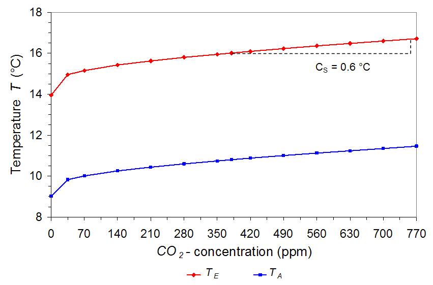
OPEN JOURNAL OF ATMOSPHERIC AND CLIMATE CHANGE
However, when assuming a reduced TSI-anomaly of ES = 0.1% over the last century, it appears
consequent, also to emanate from a smaller solar variation ES over the period 1983 - 2000. As already
stated before, this results in a larger feedback parameter s f , which at an increase of only ES = 0.05 %
over this time interval rises up to s f = 180 to further explain the observed cloud variation. A fit under
these conditions and with hC = lH =4 W /m2/ ° C gives a weighting for the thermal to solar cloud feedback
of 9/91 % with a solar fraction of 0.54 ° C and a CO2 initiated contribution of 0.2 ° C. The first part just
reflects the solar sensitivity, whereas for the equilibrium climate sensitivity we calculate CS = 0.56 ° C,
which under the above assumptions of a relatively small solar anomaly rather represents an upper limit for
this quantity. The respective plot of the temperatures TE and TA as a function of the CO2 concentration is
shown in Figure 14. In this case both graphs almost proceed parallel to each other, so that convection
only contributes to small (and under these conditions even slightly positive) feedback.
Figure 14. Calculated surface temperature TE (red) and lower tropospheric temperature TA (blue) as a function of
CO2 concentration, based on a combination of thermally and solar induced cloud feedback.
6.4 Assessment of Results
We find that in all scenarios, which include solar activities, this solar contribution to global warming is
the dominant part and under special conditions could even be up to 6x larger than the CO2 influence. This
is in clear contradiction to the IPCC, which traces the rising temperatures over the last century back to the
anthropogenic emission of GH-gases (95 % probability), whereas any noticeable solar effect is denied.
Our calculations show, that the solar part can only be pushed below the greenhouse contribution, when
the increase of the TSI over the last century is assumed to be smaller than 0.1 % and almost identical with
the variations over the period 1983 - 2000 (ES ES).
Of course, no solar influence would exist, when any solar anomaly could completely be excluded, this
over the 20th century as well as over the eighties and nineties in contradiction to Refs [35, 42, 4850, 52].
Then the worst case with respect to global warming by CO2 would be, to attribute the observed ISCCP
cloud changes only to CO2 induced thermal feedback and to exclude all other influences like the PDO,
SOI or other GH-gases. For this special and rather improbable scenario we calculate a maximum climate
44

Advanced Two-Layer Climate Model for the Assessment of Global Warming by CO2
sensitivity of CS = 1.73 ° C (see Table 7, line 23), explaining 0.6 ° C of the warming over the last century.
In spite of the maximum thermally induced cloud feedback this sensitivity still lies at the lower edge
of the IPCC data range [1], this because of the smaller water vapour feedback we deduce here, and the
inclusion of two additional processes, the convection and evaporation feedback, which are generally not
considered in the IPCC publications.
Additionally including solar activities over the last century as well as all relevant feedback processes,
we derive with a lower anomaly of ES = 0.1% a solar sensitivity of SS = 0.5 ° C and a climate sensitivity
of CS = 0.6 ° C, which are in full agreement with all constraints. Supposing a larger anomaly of ES =
0.2% the respective sensitivities would still further decline to SS = 0.3 ° C and CS = 0.4 ° C.
The largest uncertainties in all these considerations result from the cloud feedback mechanisms, and
the solar variations, which are estimated to be 50 %.
In principle our calculations confirm the investigations of Ziskin and Shaviv [42], showing the basically
strong influence of solar activities on the climate. The higher solar and therefore smaller CO2 contribution
in our case may be attributed to the fact that we use different feedback contributions and also additional
feedback processes, which for the climate sensitivity are deduced from our own calculations and for the
solar sensitivity are essentially orientated at the cloud changes in the eighties and nineties. In addition,
our calculations only represent an equilibrium state of EASy, whereas Ziskin et al. derive their data from
a multidimensional fit to the temperature evolution over the last century.
In any case, the preceding discussion makes clear, that a climate sensitivity in agreement with the IPCC
data [1] would only be possible, when any solar induced influence could be completely denied and a
strong CO2 induced thermal cloud feedback would be assumed.
7. CONCLUSION
The objective of this paper was to examine and to quantify the influence of GH-gases on our climate.
Based on the HITRAN-2008 database [4] detailed spectroscopic calculations on the absorptivities of water
vapour and the gases carbon dioxide, methane and ozone in the atmosphere are presented.
The line-by-line calculations for solar radiation from 0.18 ľm (sw radiation) as well as for the
terrestrial radiation from 3100 ľm (lw radiation) show, that due to the strong overlap of the CO2 and
CH4 spectra with water vapour lines the influence of these gases significantly declines with increasing
water vapour pressure, and that with increasing CO2-concentration well noticeable saturation effects are
observed limiting substantially the impact of CO2 on global warming.
The calculations were performed for three climate zones, the tropics, mid-latitudes and high-latitudes,
based on actual data of the water vapour content, which is considerably varying with altitude above ground
as well as with the climate zone and, therefore, with the temperature. The vertical variation in humidity
and temperature as well as in the partial gas pressures and the total pressure is considered by computing
individual absorption spectra for up to 228 atmospheric layers and then integrating from ground level up
to 86 km altitude.
The varying path length of sun light in these layers, which depends on the angle of incidence to the
atmosphere and therefore on the geographic latitude and longitude, is included by considering the Earth
as a truncated icosahedron (Bucky ball) consisting of 32 surface elements with well defined angles to the
incident radiation, and assigning each of these areas to one of the three climate zones.
45

OPEN JOURNAL OF ATMOSPHERIC AND CLIMATE CHANGE
Propagation of the long-wave radiation, in particular the up- and down-welling radiation, emitted
by the atmosphere itself, as well as their variation with temperature are derived from radiation transfer
calculations for each zone.
To identify the influence of the absorbing gases on the climate and particularly the effect of an
increasing CO2-concentration on global warming, we developed an advanced two-layer climate model,
which describes the Earth's surface and the atmosphere as two layers acting simultaneously as absorbers
and Planck radiators. Also heat transfer by convection and evaporation between these layers is considered.
At equilibrium each, the surface as well as the atmosphere, deliver as much power as they suck up from
the sun and the neighbouring layer or climate zone.
The model includes sw and lw scattering processes at the atmosphere and at clouds, in particular
considering multiple scattering between the surface and clouds. It also includes the common feedback
processes like water vapour, lapse rate and albedo feedback, but additionally takes into account the
influence of a temperature dependent sensible and latent heat flux as well as temperature induced and
solar induced cloud cover feedback.
As direct reference for the incident and outgoing fluxes in the model we use the energy and radiation
budget scheme of Tremberth et al. [20], which at a reference CO2 concentration of 380 ppm and a ground
temperature of 16 ° C can well be reproduced.
With the sw and lw absorptivities as the key parameters in such model then the surface temperature
and the lower atmospheric temperature are calculated as a function of the CO2 concentration. From the
temperature variations, found at doubled CO2 concentration, the CO2 climate sensitivity and air sensitivity
are derived.
Particularly the individual feedback processes with their different influence on the climate sensitivity
are extensively discussed. While the albedo- and to some degree the lapse rate feedback are adopted from
literature, the water vapour feedback is derived from the sw and lw absorptivity calculations over the
different climate zones. With an amplification at clear sky conditions of 1.5 and at mean cloud cover of
1.2 these values are smaller than assumed in other climate models [27, 28].
Since it is found that with increasing CO2 concentration the air temperature is less rapidly increasing
than the surface temperature, the convection at the boundary of both layers rises with the concentration.
As a consequence more thermal energy is transferred from the surface to the atmosphere. Similarly, with
increasing temperature also evaporation and precipitation are increasing with the ground temperature.
Both these effects contribute to negative feedback and are additionally included in the simulations.
A special situation is found for the influence of clouds on the radiation and energy budget. From
measurements of the global cloud cover over a period of 27 years it is deduced that the global mean
temperature is increasing with decreasing cloud cover [25]. However, it is not clear, if a lower cloud
cover is the consequence of the increasing temperature, or if the cloud cover is influenced and at least to
some degree controlled by some other mechanism, particularly solar activities. In the first case a strong
amplifying temperature induced cloud feedback had to be considered, this for the climate sensitivity as
well as for a respective solar sensitivity, whereas in the other case the temperature induced cloud effect
would disappear for both sensitivities and only a solar induced cloud feedback had to be included due to
the solar influence.
A deliberate approach which mechanism really controls the cloud cover with its dominant influence
on the climate and solar sensitivity can be derived from model simulations, which additionally include
the solar effect and compare this with the measured temperature increase over the last century. These
46

Advanced Two-Layer Climate Model for the Assessment of Global Warming by CO2
simulations, considering both effects, show that the observed global warming of 0.74 ° C [51] can only
satisfactorily be explained, when a temperature feedback on the clouds is completely excluded or only has
a minor influence. Otherwise the calculated warming would be significantly larger than observed, or the
thermally induced cloud feedback would have been overestimated. With a combination of temperature and
solar induced cloud feedback we deduce a CO2 climate sensitivity of CS = 0.6 ° C and a solar sensitivity,
related to 0.1 % change of the solar constant, of SS = 0.5 ° C. An increase in the solar activity of only 0.1
% over 100 years then contributes to a warming of 0.54 ° C, and the 100 ppm increase of CO2 over this
period causes additional 0.2 ° C in excellent agreement with the measured warming and cloud cover.
From our investigations, which are based on actual spectroscopic data and which consider all relevant
feedback processes as well as the solar influence, we can conclude, that a CO2 climate sensitivity larger
1 ° C seems quite improbable, whereas a value of 0.5 - 0.7 ° C - depending on the considered solar anomaly
- fits well with all observations of a changing solar constant, the cloud cover and global temperature. A
climate sensitivity in agreement with the IPCC specifications (1.5 - 4.5 ° C) would only be possible, when
any solar influence could completely be excluded, and only CO2 induced thermal cloud feedback would
be assumed, then yielding a value of 1.7 ° C.
It should be noticed that different to global circulation models, which try to predict local climate
variations over some time period and, therefore, have to solve complex coupled nonlinear differential
equations with countless parameters, for tracing the climate sensitivity this is of no significance. We
calculate an equilibrium state and can average over larger local variations, for which a partitioning into
three climate zones is quite sufficient. In addition, a simple energy balance model, focussing on the main
physical processes, is much more transparent than any AOGCM and can help to better understand the
complex interrelations characterizing our climate system.
References
[1] IPCC, "Summary for Policymakers," Climate Change 2013: The Physical Science Basis. Contribu-
tion of Working Group I to the Fifth Assessment Report of the Intergovernmental Panel on Climate
Change [T.F. Stocker, D. Qin, G.-K. Plattner, M. Tignor, S.K. Allen, J. Boschung, A. Nauels, Y. Xia, V.
Bex and P.M. Midgley (eds.)]. Cambridge University Press, Cambridge, United Kingdom and New
York, NY, USA, 2013.
[2] D. Randall, R. Wood, S. Bony, R. Colman, T. Fichefet, J. Fyfe, V. Kattsov, A. Pitman, J. Shukla,
J. Srinivasan, et al., "Climate Models and Their Evaluation," Climate Change 2007: The Physical
Science Basis. Contribution of Working Group I to the Fourth Assessment Report of the Intergov-
ernmental Panel on Climate Change [Solomon, S., D. Qin, M. Manning, Z. Chen, M. Marquis, K.B.
Averyt, M.Tignor and H.L. Miller (eds.)]. Cambridge University Press, Cambridge, United Kingdom
and New York, NY, USA, 2007.
[3] IPCC, "Climate Change 2001: The Scientific Basis," Contribution of Working Group 1 to the Third
Assessment Report of the Intergovernmental Panel on Climate Change, edited by J. T. Houghton, Y.
Ding, D. J. Griggs, M. Noguer, P. J. van der Linden, X. Dai, K. Maskell and C. A. Johnson (eds).
Cambridge University Press, Cambridge, UK, and New York, USA, chapter 6: Radiative Forcing of
Climate Change, p. 354, 2001.
[4] L. S. Rothman, I. E. Gordon, A. Barbe, D. C. Benner, P. F. Bernath, M. Birk, V. Boudon, L. R.
Brown, A. Campargue, J.-P. Champion, et al., "The HITRAN 2008 molecular spectroscopic database,"
Journal of Quantitative Spectroscopy and Radiative Transfer, vol. 110, no. 9, pp. 533572, 2009.
47

OPEN JOURNAL OF ATMOSPHERIC AND CLIMATE CHANGE
[5] R. M. Goody and Y. L. Yung, Atmospheric Radiation: Theoretical Basis, 2nd ed. New York, NY:
Oxford University Press, 1989.
[6] M. L. Salby, Physics of the Atmosphere and Climate. Cambridge University Press, 2012.
[7] H. Harde, "Radiation and Heat Transfer in the Atmosphere: A Comprehensive Approach on a
Molecular Basis," International Journal of Atmospheric Sciences, vol. 2013. http://dx.doi.
org/10.1155/2013/503727.
[8] L. S. Rothman, C. Rinsland, A. Goldman, S. Massie, D. Edwards, J. Flaud, A. Perrin, C. Camy-Peyret,
V. Dana, J.-Y. Mandin, et al., "The HITRAN Molecular Spectroscopic Database and HAWKS; 1996
Edition," Journal of Quantitative Spectroscopy and Radiative Transfer, vol. 60, no. 5, pp. 665710,
1998.
[9] US Standard Atmosphere, "National Oceanic and Atmospheric Administration, National Aeronautics
and Space Administration," tech. rep., Washington D.C., 1976.
[10] S. Vey, Bestimmung und Analyse des atmosph¨arischen Wasserdampfgehaltes aus globalen GPS-
Beobachtungen einer Dekade mit besonderem Blick auf die Antarktis. PhD thesis, Technical
University Dresden, 2007.
[11] H. Harde, Was tr¨agt CO2 wirklich zur globalen Erw¨armung bei? Spektroskopische Untersuchungen
und Modellrechnungen zum Einfluss von H2O, CO2, CH4 und O3 auf unser Klima. Books on
Demand, Norderstedt, 2011. ISBN: 9 783842 371576.
[12] H. Harde and J. Pfuhl, "MolExplorer A Program-Platform for the Calculation of Molecular Spectra
and Radiation Transfer in the Atmosphere," 20062014.
[13] K. Schwarzschild, "G¨ottinger Nachrichten," p. 41, 1906.
[14] R. Hanel, B. Conrath, V. Kunde, C. Prabhakara, I. Revah, V. Salomonson, and G. Wolford, "The
Nimbus 4 Infrared Spectroscopy Experiment, 1. Calibrated Thermal Emission Spectra," Journal of
Geophysical Research, vol. 77, no. 15, pp. 26292641, 1972.
[15] B. Barkstrom, E. Harrison, G. Smith, R. Green, J. Kibler, R. Cess, and the ERBE Science Team,
"Earth Radiation Budget Experiment(ERBE) archival and April 1985 results," Bulletin of the Ameri-
can Meteorological Society, vol. 70, no. 10, pp. 12541262, 1989.
[16] T. D. Bess and G. L. Smith, "Earth radiation budget: Results of outgoing longwave radiation
from Nimbus-7, NOAA-9, and ERBS satellites," Journal of Applied Meteorology, vol. 32, no. 5,
pp. 813824, 1993.
[17] B. A. Wielicki, B. R. Barkstrom, E. F. Harrison, R. B. Lee III, G. Louis Smith, and J. E. Cooper,
"Clouds and the Earth's Radiant Energy System (CERES): An earth observing system experiment,"
Bulletin of the American Meteorological Society, vol. 77, no. 5, pp. 853868, 1996.
[18] B. A. Wielicki, K. Priestley, P. Minnis, N. Loeb, D. Kratz, T. Charlock, D. Doelling, and D. Young,
"CERES radiation budget accuracy overview," in Preprints, 12th Conf. on Atmospheric Radiation,
Madison, WI, Amer. Meteor. Soc, vol. 9, 2006.
[19] T. Wong, B. A. Wielicki, R. B. Lee III, G. L. Smith, K. A. Bush, and J. K. Willis, "Re-examination
of the observed decadal variability of Earth Radiation Budget using altitude-corrected ERBE/ERBS
nonscanner WFOV data," Journal of Climate, vol. 19, no. 16, pp. 40284040, 2006.
[20] K. E. Trenberth, J. T. Fasullo, and J. Kiehl, "Earths Global Energy Budget," Bulletin of the American
Meteorological Society, vol. 90, no. 3, pp. 311323, 2009.
[21] D. D. Turner, E. J. Mlawer, G. Bianchini, M. P. Cadeddu, S. Crewell, J. S. Delamere, R. O. Knuteson,
G. Maschwitz, M. Mlynzcak, S. Paine, et al., "Ground-based high spectral resolution observations
of the entire terrestrial spectrum under extremely dry conditions," Geophysical Research Letters,
vol. 39, no. 10, 2012.
[22] W. Dines, "The heat balance of the atmosphere," Quarterly Journal of the Royal Meteorological
Society, vol. 43, no. 182, pp. 151158, 1917.
48

Advanced Two-Layer Climate Model for the Assessment of Global Warming by CO2
[23] K. N. Liou, An Introduction to Atmospheric Radiation, 2nd ed, vol. 84. Academic Press, San Diego,
CA, 2002.
[24] R. Link and H.-J. L¨udecke, "A new basic 1-dimensional 1-layer model obtains excellent agreement
with the observed Earth temperature," Int. J. Modern Physics C, vol. 22, pp. 449455, 2011.
[25] International Satellite Cloud Climatology Project(ISCCP) http://isccp.giss.nasa.gov/
products/onlineData.html or http://www.climate4you.com/index.htm.
[26] D. L. Hartmann, Global Physical Climatology, vol. 56. Academic Press, New York, 1994.
[27] Reference 2, section 8.6.3.
http://www.ipcc.ch/publications_and_data/ar4/
wg1/en/ch8s8-6-3-1.html.
[28] B. J. Soden and I. M. Held, "An assessment of climate feedbacks in coupled ocean-atmosphere
models," Journal of Climate, vol. 19, no. 14, pp. 33543360, 2006.
[29] R. S. Lindzen, M.-D. Chou, and A. Y. Hou, "Does the Earth have an adaptative infrared iris?,"
Bulletin of the American Meteorological Society, vol. 82, no. 3, pp. 417432, 2001.
[30] B. A. Laken and E. Pall´e, "Understanding sudden changes in cloud amount: The Southern Annular
Mode and South American weather fluctuations," Journal of Geophysical Research: Atmospheres,
vol. 117, no. D13, pp. 19842012, 2012.
[31] H. Cho, C.-H. Ho, and Y.-S. Choi, "The observed variation in cloud-induced longwave radiation
in response to sea surface temperature over the Pacific warm pool from MTSAT-1R imagery,"
Geophysical Research Letters, vol. 39, no. 18, 2012.
[32] P. M. Caldwell, Y. Zhang, and S. A. Klein, "CMIP3 Subtropical Stratocumulus Cloud Feedback
Interpreted Through a Mixed-Layer Model," Journal of Climate, 2012.
[33] R. W. Spencer and W. D. Braswell, "On the Misdiagnosis on Surface Temperature Feedbacks from
Variations in Earth's Radiant Energy Balance," Remote Sensing, vol. 3, no. 8, pp. 16031613, 2011.
[34] J.-R. Petit, J. Jouzel, D. Raynaud, N. I. Barkov, J.-M. Barnola, I. Basile, M. Bender, J. Chappellaz,
M. Davis, G. Delaygue, et al., "Climate and Atmospheric History of the past 420,000 Years from the
Vostok Ice Core, Antarctica," Nature, vol. 399, no. 6735, pp. 429436, 1999.
[35] R. C. Willson and A. V. Mordvinov, "Secular Total Solar Irradiance Trend During Solar Cycles 21 -
23," Geophysical Research Letters, vol. 30, no. 5, pp. 14, 2003.
[36] H. Svensmark, "Influence of Cosmic Rays on Earth's Climate," Physical Review Letters, vol. 81,
no. 22, pp. 50275030, 1998.
[37] H. Svensmark, J. O. P. Pedersen, N. D. Marsh, M. B. Enghoff, and U. I. Uggerhřj, "Experimental
Evidence for the Role of Ions in Particle Nucleation under Atmospheric Conditions," Proceedings
of the Royal Society A: Mathematical, Physical and Engineering Science, vol. 463, no. 2078,
pp. 385396, 2007.
[38] H. Svensmark, T. Bondo, and J. Svensmark, "Cosmic Ray Decreases affect Atmospheric Aerosols
and Clouds," Geophysical Research Letters, vol. 36, no. 15, pp. 14, 2009.
[39] M. B. Enghoff, J. O. P. Pedersen, U. I. Uggerhřj, S. M. Paling, and H. Svensmark, "Aerosol
Nucleation Induced by a High Energy Particle Beam," Geophysical Research Letters, vol. 38, no. 9,
pp. 14, 2011.
[40] J. Kirkby, J. Curtius, J. Almeida, E. Dunne, J. Duplissy, S. Ehrhart, A. Franchin, S. Gagn´e, L. Ickes,
A. K¨urten, et al., "Role of Sulphuric Acid, Ammonia and Galactic Cosmic Rays in Atmospheric
Aerosol Nucleation," Nature, vol. 476, no. 7361, pp. 429435, 2011.
[41] F. Vahrenholt and S. L¨uning, Die kalte Sonne. Hoffmann und Campe Verlag, Hamburg, 2012.
[42] S. Ziskin and N. J. Shaviv, "Quantifying the role of solar radiative forcing over the 20th century,"
Advances in Space Research, vol. 50, no. 6, pp. 762776, 2012.
[43] J. D. Haigh, "The role of stratospheric ozone in modulating the solar radiative forcing of climate,"
Nature, vol. 370, no. 6490, pp. 544546, 1994.
49

OPEN JOURNAL OF ATMOSPHERIC AND CLIMATE CHANGE
[44] J. D. Haigh, "The impact of solar variability on climate," Science, vol. 272, no. 5264, pp. 981984,
1996.
[45] J. D. Haigh, A. R. Winning, R. Toumi, and J. W. Harder, "An influence of solar spectral variations
on radiative forcing of climate," Nature, vol. 467, no. 7316, pp. 696699, 2010.
[46] J. Kristj´ansson, J. Kristiansen, and E. Kaas, "Solar activity, cosmic rays, clouds and climate: An
update," Advances in Space Research, vol. 34, no. 2, pp. 407415, 2004.
[47] M. Voiculescu, I. G. Usoskin, and K. Mursula, "Different response of clouds to solar input," Geo-
physical Research Letters, vol. 33, no. 21, 2006.
[48] A. Shapiro, W. Schmutz, E. Rozanov, M. Schoell, M. Haberreiter, A. Shapiro, and S. Nyeki, "A
New Approach to Long-Term Reconstruction of the Solar Irradiance Leads to Large Historical Solar
Forcing," Astronomy & Astrophysics,, vol. 529, pp. 18, 2011.
[49] D. V. Hoyt and K. H. Schatten, "Group Sunspot Numbers: A new solar activity reconstruction,"
Solar Physics, vol. 179, p. 189, 1998.
[50] I. Usoskin, G. Hulot, Y. Gallet, R. Roth, A. Licht, F. Joos, G. Kovaltsov, E. Th´ebault, and A. Khokhlov,
"Evidence for distinct modes of solar activity," Astronomy & Astrophysics, vol. 562, 2014.
[51] Goddard Institute for Space Studies. http://data.giss.nasa.gov/gistemp/graphs.
[52] X. ZHAO and X. FENG, "Periodicities of solar activity and the surface temperature variation of the
Earth and their correlations," Chinese Science Bulletin, vol. 59, no. 14, pp. 12841292, 2014.
[53] T. Wenzler, S. Solanki, and N. Krivova, "Reconstructed and measured total solar irradiance: Is there
a secular trend between 1978 and 2003?," Geophysical Research Letters, vol. 36, no. 11, 2009.
50

Document Outline

INTRODUCTION
SPECTROSCOPIC CALCULATIONS
- Fundamentals
  - Integral Absorptivity
  - Atmospheric Pressure and Temperature Changes
  - Concentration of Greenhouse Gases
- Short-Wave Absorption in the Atmosphere
  - Path Length in the Atmosphere
  - Absorption Spectrum
- Long-Wave Absorption in the Atmosphere
  - Spectral Range and Number of Lines
  - Propagation of Terrestrial Radiation
  - Absorption Spectrum
RADIATION TRANSFER IN THE ATMOSPHERE
- Radiation Transfer Equation for the Spectral Radiance
- Radiation Transfer Equation for the Spectral Intensity
- Radiation Transfer Calculations
ADVANCED TWO-LAYER CLIMATE MODEL
- Short-Wave Radiation Budget
- Long-Wave Radiation Budget
- Sensible and Latent Heat
- Total Radiation and Energy Budget
SIMULATIONS WITHOUT SOLAR INFLUENCE
- Adaptation to Satellite Measurements
- Influence of some Model-Parameters on the Balance
- Direct Influence of CO2 on the Surface-Temperature
- Feedback Processes
  - Water-Vapour-Feedback
  - Lapse-Rate-Feedback
  - Earth Albedo Feedback
  - Convection Feedback
  - Evaporation Feedback
  - Thermally Induced Cloud Feedback
  - Total Feedback
SIMULATIONS AND RESULTS WITH SOLAR INFLUENCE
- Solar Induced Cloud Feedback
- Thermally Induced Cloud Feedback
- Combined Thermal- and Solar-Induced Feedback
- Assessment of Results
CONCLUSION
References